Approximating functions on R^2
Contents
Approximating functions on \(R^2\)
Randall Romero Aguilar, PhD
This demo is based on the original Matlab demo accompanying the Computational Economics and Finance 2001 textbook by Mario Miranda and Paul Fackler.
Original (Matlab) CompEcon file: demapp02.m
Running this file requires the Python version of CompEcon. This can be installed with pip by running
!pip install compecon --upgrade
Last updated: 2022-Oct-22
About
This notebook illustrates how to use CompEcon Toolbox routines to construct and operate with an approximant for a function defined on a rectangle in \(R^2\).
In particular, we construct an approximant for \(f(x_1,x_2) = \frac{\cos(x_1)}{\exp(x_2)}\) on \([-1,1]\times[-1,1]\). The function used in this illustration posseses a closed-form, which will allow us to measure approximation error precisely. Of course, in practical applications, the function to be approximated will not possess a known closed-form.
In order to carry out the exercise, one must first code the function to be approximated at arbitrary points. Let’s begin:
Initial tasks
import numpy as np
import pandas as pd
import matplotlib.pyplot as plt
from compecon import BasisChebyshev, BasisSpline, nodeunif
from matplotlib import cm
Defining some functions
Function to be approximated and analytic partial derivatives
exp, cos, sin = np.exp, np.cos, np.sin

f   = lambda x:  cos(x[0]) / exp(x[1])
d1  = lambda x: -sin(x[0]) / exp(x[1])
d2  = lambda x: -cos(x[0]) / exp(x[1])
d11 = lambda x: -cos(x[0]) / exp(x[1])
d12 = lambda x:  sin(x[0]) / exp(x[1])
d22 = lambda x:  cos(x[0]) / exp(x[1])
Set the points of approximation interval:
a, b = 0, 1
Choose an approximation scheme.
In this case, let us use an 6 by 6 Chebychev approximation scheme:
n = 6  # order of approximation
basis = BasisChebyshev([n, n], a, b)
# write n twice to indicate the two dimensions.
# a and b are broadcast.
Compute the basis coefficients c.
There are various way to do this:
One may compute the standard approximation nodes
xand corresponding interpolation matrixPhiand function valuesyand use:
x = basis.nodes
Phi = basis.Phi(x)  # input x may be omitted if evaluating at the basis nodes
y = f(x)
c = np.linalg.solve(Phi, y)
Alternatively, one may compute the standard approximation nodes
xand corresponding function valuesyand use these values to create aBasisChebyshevobject with keyword argumenty:
x = basis.nodes
y = f(x)
fa = BasisChebyshev([n, n], a, b, y=y)
# coefficients can be retrieved by typing fa.c
… or one may simply pass the function directly to BasisChebyshev using keyword
f, which by default will evaluate it at the basis nodes
F = BasisChebyshev([n, n], a, b, f=f)
# coefficients can be retrieved by typing F.c
Evaluate the basis
Having created a BasisChebyshev object, one may now evaluate the approximant at any point x by calling the object:
x = np.array([[0.5],[0.5]]) # first dimension should match the basis dimension
F(x)
0.5322807350499545
… one may also evaluate the approximant’s first partial derivatives at x:
dfit1 = F(x, [1, 0])
dfit2 = F(x, [0, 1])
… one may also evaluate the approximant’s second own partial and cross partial derivatives at x:
dfit11 = F(x, [2, 0])
dfit22 = F(x, [0, 2])
dfit12 = F(x, [1, 1])
Compare analytic and numerical computations
print('Function Values and Derivatives of cos(x_1)/exp(x_2) at x=(0.5,0.5)')

results = pd.DataFrame({
    'Numerical': [F(x),dfit1,dfit2,dfit11, dfit12,dfit22],
    'Analytic': np.r_[f(x), d1(x), d2(x), d11(x), d12(x), d22(x)]},
    index=['Function', 'Partial 1','Partial 2','Partial 11','Partial 12', 'Partial 22']
)
results.round(5)
Function Values and Derivatives of cos(x_1)/exp(x_2) at x=(0.5,0.5)
| Numerical | Analytic | |
|---|---|---|
| Function | 0.53228 | 0.53228 |
| Partial 1 | -0.29079 | -0.29079 |
| Partial 2 | -0.53228 | -0.53228 |
| Partial 11 | -0.53223 | -0.53228 |
| Partial 12 | 0.29079 | 0.29079 |
| Partial 22 | 0.53223 | 0.53228 |
The cell below shows how the preceeding table could be generated in a single loop, using the zip function and computing all partial derivatives at once.
labels = ['Function', 'Partial 1','Partial 2','Partial 11','Partial 12','Partial 22']
analytics =[func(x) for func in [f,d1,d2,d11,d12,d22]]
deriv = [[0, 1, 0, 2, 0, 1],
         [0, 0, 1, 0, 2, 1]]

ff = '%-11s %12.5f  %12.5f'
print('Function Values and Derivatives of cos(x_1)/exp(x_2) at x=(0.5,0.5)')
print('%-11s %12s  %12s\n' % ('','Numerical', 'Analytic'), '_'*40)
for lab,appr,an in zip(labels, F(x,order=deriv),analytics):
    print(f'{lab:11s} {an[0]:12.5f} {appr:12.5f}')
Function Values and Derivatives of cos(x_1)/exp(x_2) at x=(0.5,0.5)
               Numerical      Analytic
 ________________________________________
Function         0.53228      0.53228
Partial 1       -0.29079     -0.29079
Partial 2       -0.53228     -0.53228
Partial 11      -0.53228     -0.53223
Partial 12       0.29079      0.53223
Partial 22       0.53228      0.29079
Approximation accuracy
One may evaluate the accuracy of the Chebychev polynomial approximant by computing the approximation error on a highly refined grid of points:
nplot = [101, 101]         # chose grid discretization
X = nodeunif(nplot, [a, a], [b, b])  # generate refined grid for plotting
yapp = F(X)        # approximant values at grid nodes
yact = f(X)                      # actual function values at grid points
error = (yapp - yact).reshape(nplot)
X1, X2 = X
X1.shape = nplot
X2.shape = nplot

fig1 = plt.figure(figsize=[12, 6])
ax = fig1.add_subplot(1, 1, 1, projection='3d')
ax.plot_surface(X1, X2, error, rstride=1, cstride=1, cmap=cm.coolwarm,
                linewidth=0, antialiased=False)
ax.set_xlabel('$x_1$')
ax.set_ylabel('$x_2$')
ax.set_zlabel('error')
ax.set_title('Chebychev Approximation Error')
ax.ticklabel_format(style='sci', axis='z', scilimits=(-1,1))
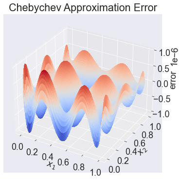
The plot indicates that an order 11 by 11 Chebychev approximation scheme produces approximation errors no bigger in magnitude than \(10^{-10}\).
Let us repeat the approximation exercise, this time constructing an order 21 by 21 cubic spline approximation scheme:
n = [21, 21]                          # order of approximation
S = BasisSpline(n, a, b, f=f)
yapp = S(X)        # approximant values at grid nodes
error = (yapp - yact).reshape(nplot)

fig2 = plt.figure(figsize=[12, 6])
ax = fig2.add_subplot(1, 1, 1, projection='3d')
ax.plot_surface(X1, X2, error, rstride=1, cstride=1, cmap=cm.coolwarm,
                linewidth=0, antialiased=False)
ax.set_xlabel('$x_1$')
ax.set_ylabel('$x_2$')
ax.set_zlabel('error')
ax.set_title('Cubic Spline Approximation Error');
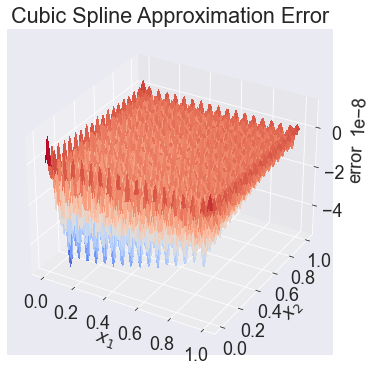
The plot indicates that an order 21 by 21 cubic spline approximation scheme produces approximation errors no bigger in magnitude than \(10^{-6}\).