Asset Replacement Model
Contents
Asset Replacement Model
Randall Romero Aguilar, PhD
This demo is based on the original Matlab demo accompanying the Computational Economics and Finance 2001 textbook by Mario Miranda and Paul Fackler.
Original (Matlab) CompEcon file: demdp02.m
Running this file requires the Python version of CompEcon. This can be installed with pip by running
!pip install compecon --upgrade
Last updated: 2022-Oct-22
About
Profit-maximizing entrepreneur must decide when to replace an aging asset.
import numpy as np
import matplotlib.pyplot as plt
from compecon import BasisSpline, DPmodel, qnwnorm, NLP
Model Parameters
The maximum age of the asset is \(A=6\), production function coefficients are \(\alpha =[50.0, -2.5, -2.5]\), net replacement cost is \(\kappa = 40\), long-run mean unit profit is \(\bar{p} = 1\), the unit profit autoregression coefficient is \(\gamma = 0.5\), the standard deviation of unit profit shock is \(\sigma = 0.15\), and the discount factor is \(\delta = 0.9\).
A   = 6
ɑ   = np.array([50, -2.5, -2.5])
κ   = 40
pbar= 1.0
ɣ   = 0.5
σ   = 0.15
δ   = 0.9
State space
The state variables are the current unit profit \(p\) (continuous) and the age of asset \(a\in\{1,2,\dots,A\}\).
dstates = [f'a={age+1:d}' for age in range(A)]
print('Discrete states are :', dstates)
Discrete states are : ['a=1', 'a=2', 'a=3', 'a=4', 'a=5', 'a=6']
Here, we approximate the unit profit with a cubic spline basis of \(n=200\) nodes, over the interval \(p\in[0,2]\).
n  = 200
pmin, pmax = 0.0, 2.0
basis = BasisSpline(n, pmin, pmax, labels=['unit profit'])
Action space
There is only one choice variable \(j\): whether to keep(0) or replace(1) the asset.
options = ['keep', 'replace']
Reward Function
The instant profit depends on the asset age and whether it is replaced. An asset of age \(a=A\) must be replaced. If the asset is replaced, the profit is \(50p\) minus the cost of replacement \(\kappa\); otherwise the profit depends on the age of the asset, \((\alpha_0 + \alpha_1 a + \alpha_2 a^2)p\).
def profit(p, x, i, j):
    a = i + 1
    if j or a == A:
        return p * 50 - κ
    else:
        return p * (ɑ[0] + ɑ[1]*a + ɑ[2]*a**2 )
State Transition Function
The unit profit \(p\) follows a Markov Process
where \(\epsilon \sim N(0,\sigma^2)\).
def transition(p, x, i, j, in_, e):
    return pbar + ɣ * (p - pbar) + e
The continuous shock must be discretized. Here we use Gauss-Legendre quadrature to obtain nodes and weights defining a discrete distribution that matches the first 10 moments of the Normal distribution (this is achieved with \(m=5\) nodes and weights).
m = 5
e, w = qnwnorm(m,0,σ**2)
On the other hand, the age of the asset is deterministic: if it is replaced now it will be new (\(a=0\)) next period; otherwise its age will be \(a+1\) next period if current age is \(a\).
h = np.zeros((2, A),int)
h[0, :-1] = np.arange(1, A)
Model Structure
model = DPmodel(basis, profit, transition,
                i=dstates,
                j=options,
                discount=δ, e=e, w=w, h=h)
SOLUTION
The solve method returns a pandas DataFrame.
S = model.solve()
S.head()
Solving infinite-horizon model collocation equation by Newton's method
iter change       time
------------------------------
0 3.7e+02 0.1952
1 4.3e+01 0.5473
2 1.2e+01 1.1229
3 5.7e-01 1.6491
   4       4.5e-13    2.0834
Elapsed Time =    2.08 Seconds
| unit profit | i | value | resid | j* | value[keep] | value[replace] | ||
|---|---|---|---|---|---|---|---|---|
| unit profit | ||||||||
| a=1 | 0.000000 | 0.000000 | 0 | 234.982583 | -5.684342e-14 | keep | 234.982583 | 206.124123 |
| 0.001001 | 0.001001 | 0 | 235.058576 | -6.159590e-07 | keep | 235.058576 | 206.209036 | |
| 0.002001 | 0.002001 | 0 | 235.134563 | -6.366804e-07 | keep | 235.134563 | 206.293949 | |
| 0.003002 | 0.003002 | 0 | 235.210544 | -2.317537e-07 | keep | 235.210544 | 206.378862 | |
| 0.004002 | 0.004002 | 0 | 235.286520 | 4.292312e-07 | keep | 235.286520 | 206.463774 |
Analysis
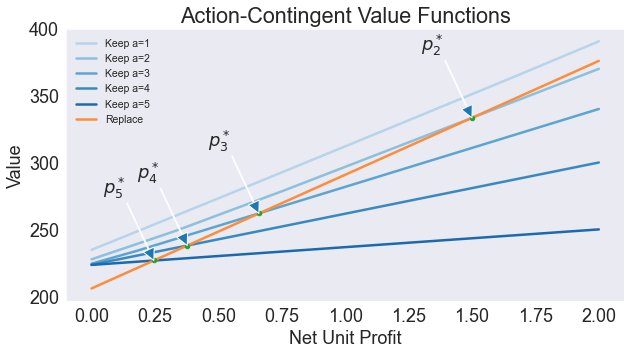
Plot Action-Contingent Value Functions
# Compute and Plot Critical Unit Profit Contributions
pcrit = [NLP(lambda s: model.Value_j(s)[i].dot([1,-1])).broyden(0.0) for i in range(A-1)]
vcrit = [model.Value(s)[i] for i, s in enumerate(pcrit)]
fig1, ax = plt.subplots(figsize=[10,5])

ax.set(title='Action-Contingent Value Functions', xlabel='Net Unit Profit',ylabel='Value')

cc = np.linspace(0.3,0.9,model.dims.ni)


for a, i in enumerate(dstates[:-1]):
    ax.plot(S.loc[i,'value[keep]'] ,color=plt.cm.Blues(cc[a]), label=f'Keep {i}')

ax.plot(S.loc['a=1','value[replace]'], color=plt.cm.Oranges(0.5),label='Replace')

for a, i in enumerate(dstates[:-1]):
    if pmin < pcrit[a] < pmax:
        ax.plot(pcrit[a], vcrit[a], color='C2', marker='.', markersize=9)
        ax.annotate(f'$p^*_{a+1}$', (pcrit[a], vcrit[a]), xytext=(pcrit[a]-0.2, vcrit[a]+50), arrowprops=dict(width=1))
        print(f'Age {a+1:d}  Profit {pcrit[a]:5.2f}')

ax.legend(fontsize="xx-small")
Age 2  Profit  1.50
Age 3  Profit  0.66
Age 4  Profit  0.38
Age 5  Profit  0.25
<matplotlib.legend.Legend at 0x13462c93d00>
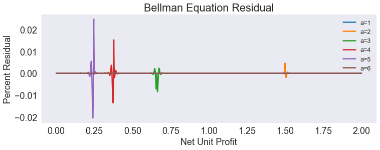
Plot Residual
fig, ax = plt.subplots(1,1, figsize=[12,4])
S['resid2'] = 100*S['resid'] / S['value']
S['resid2'].unstack(level=0).plot(ax=ax)
ax.set(title='Bellman Equation Residual',
       xlabel='Net Unit Profit',
       ylabel='Percent Residual')

ax.legend(fontsize="x-small")
<matplotlib.legend.Legend at 0x13462e22130>
SIMULATION
T = 50
nrep = 10000
sinit = np.full(nrep, pbar)
iinit = 0
data = model.simulate(T,sinit,iinit, seed=945)
data['age'] = data.i.cat.codes + 1
Print Ergodic Moments
frm = '\t{:<10s} = {:5.2f}'

print('\nErgodic Means')
print(frm.format('Price', data['unit profit'].mean()))
print(frm.format('Age', data['age'].mean()))
print('\nErgodic Standard Deviations')
print(frm.format('Price', data['unit profit'].std()))
print(frm.format('Age', data['age'].std()))
Ergodic Means
	Price      =  1.00
	Age        =  2.01

Ergodic Standard Deviations
	Price      =  0.17
	Age        =  0.83
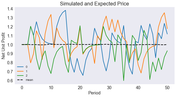
Plot Simulated and Expected Continuous State Path
data.head()
| time | _rep | i | unit profit | j* | age | |
|---|---|---|---|---|---|---|
| 0 | 0 | 0 | a=1 | 1.0 | keep | 1 |
| 1 | 0 | 1 | a=1 | 1.0 | keep | 1 |
| 2 | 0 | 2 | a=1 | 1.0 | keep | 1 |
| 3 | 0 | 3 | a=1 | 1.0 | keep | 1 |
| 4 | 0 | 4 | a=1 | 1.0 | keep | 1 |
subdata = data.query('_rep < 3').set_index(['time','_rep']).unstack()
subdata.head()
| i | unit profit | j* | age | |||||||||
|---|---|---|---|---|---|---|---|---|---|---|---|---|
| _rep | 0 | 1 | 2 | 0 | 1 | 2 | 0 | 1 | 2 | 0 | 1 | 2 |
| time | ||||||||||||
| 0 | a=1 | a=1 | a=1 | 1.000000 | 1.000000 | 1.000000 | keep | keep | keep | 1 | 1 | 1 |
| 1 | a=2 | a=2 | a=2 | 1.000000 | 1.000000 | 1.000000 | keep | keep | keep | 2 | 2 | 2 |
| 2 | a=3 | a=3 | a=3 | 1.000000 | 1.000000 | 1.000000 | replace | replace | replace | 3 | 3 | 3 |
| 3 | a=1 | a=1 | a=1 | 1.203344 | 0.796656 | 1.203344 | keep | keep | keep | 1 | 1 | 1 |
| 4 | a=2 | a=2 | a=2 | 1.101672 | 0.898328 | 1.101672 | keep | keep | keep | 2 | 2 | 2 |
fig3, ax = plt.subplots()

subdata['unit profit'].plot(ax=ax, legend=None)
ax.set(title='Simulated and Expected Price', xlabel='Period',ylabel='Net Unit Profit')

ax.plot(data[['time','unit profit']].groupby('time').mean(),'k--',label='mean')
ax.legend(fontsize="x-small")
<matplotlib.legend.Legend at 0x13462e96550>
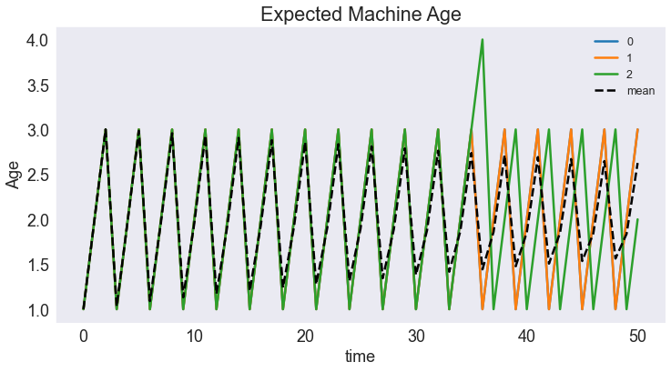
Plot Expected Discrete State Path
fig4, ax = plt.subplots()

ax.set(title='Expected Machine Age', xlabel='Period', ylabel='Age')


subdata['age'].plot(ax=ax, legend=None)
ax.plot(data[['time','age']].groupby('time').mean(),'k--',label='mean')
ax.legend(fontsize="x-small")
<matplotlib.legend.Legend at 0x13462f65be0>