Job Search Model
Contents
Job Search Model
Randall Romero Aguilar, PhD
This demo is based on the original Matlab demo accompanying the Computational Economics and Finance 2001 textbook by Mario Miranda and Paul Fackler.
Original (Matlab) CompEcon file: demdp04.m
Running this file requires the Python version of CompEcon. This can be installed with pip by running
!pip install compecon --upgrade
Last updated: 2022-Oct-22
About
Infinitely-lived worker must decide whether to quit, if employed, or search for a job, if unemployed, given prevailing market wages.
States
w prevailing wage
i unemployed (0) or employed (1) at beginning of period
Actions
j idle (0) or active (i.e., work or search) (1) this period
Parameters
Parameter |
Meaning |
|---|---|
\(v\) |
benefit of pure leisure |
\(\bar{w}\) |
long-run mean wage |
\(\gamma\) |
wage reversion rate |
\(p_0\) |
probability of finding job |
\(p_1\) |
probability of keeping job |
\(\sigma\) |
standard deviation of wage shock |
\(\delta\) |
discount factor |
Preliminary tasks
import numpy as np
import pandas as pd
import matplotlib.pyplot as plt
from compecon import BasisSpline, DPmodel, qnwnorm
FORMULATION
Worker’s reward
The worker’s reward is:
\(w\) (the prevailing wage rate), if he’s employed and active (working)
\(u=90\), if he’s unemployed but active (searching)
\(v=95\), if he’s idle (quit if employed, not searching if unemployed)
u     =  90
v     =  95

def reward(w, x, employed, active):
    if active:
        return w.copy() if employed else np.full_like(w, u)  # the copy is critical!!! otherwise it passes a pointer to w!!
    else:
        return np.full_like(w, v)
Model dynamics
Stochastic Discrete State Transition Probabilities
An unemployed worker who is searching for a job has a probability \(p_0=0.2\) of finding it, while an employed worker who doesn’t want to quit his job has a probability \(p_1 = 0.9\) of keeping it. An idle worker (someone who quits or doesn’t search for a job) will definitely be unemployed next period. Thus, the transition probabilities are
p0    = 0.20
p1    = 0.90

q = np.zeros((2, 2, 2))
q[1, 0, 1] = p0
q[1, 1, 1] = p1
q[:, :, 0] = 1 - q[:, :, 1]
Stochastic Continuous State Transition
Assuming that the wage rate \(w\) follows an exogenous Markov process
where \(\bar{w}=100\) and \(\gamma=0.4\).
wbar  = 100
ɣ = 0.40
def transition(w, x, i, j, in_, e):
    return wbar + ɣ * (w - wbar) + e
Here, \(\epsilon\) is normal \((0,\sigma^2)\) wage shock, where \(\sigma=5\). We discretize this distribution with the function qnwnorm.
σ = 5
m = 15
e, w = qnwnorm(m, 0, σ**2)
Approximation Structure
To discretize the continuous state variable, we use a cubic spline basis with \(n=150\) nodes between \(w_\text{min}=0\) and \(w_\text{max}=200\).
n = 150
wmin = 0
wmax = 200
basis = BasisSpline(n, wmin, wmax, labels=['wage'])
SOLUTION
To represent the model, we create an instance of DPmodel. Here, we assume a discout factor of \(\delta=0.95\).
model = DPmodel(basis, reward, transition,
                i =['unemployed', 'employed'],
                j = ['idle', 'active'],
                discount=0.95, e=e, w=w, q=q)
Then, we call the method solve to solve the Bellman equation
S = model.solve(show=True)
S.head()
Solving infinite-horizon model collocation equation by Newton's method
iter change       time
------------------------------
   0       2.1e+03    0.1720
1 3.5e+01 0.4380
2 1.9e+01 0.6730
3 1.4e+00 0.9291
   4       2.8e-12    1.1958
Elapsed Time =    1.20 Seconds
| wage | i | value | resid | j* | value[idle] | value[active] | ||
|---|---|---|---|---|---|---|---|---|
| wage | ||||||||
| unemployed | 0.000000 | 0.000000 | 0 | 1911.101186 | 0.000000e+00 | idle | 1911.101186 | 1906.101213 |
| 0.133422 | 0.133422 | 0 | 1911.101997 | -1.405169e-10 | idle | 1911.101997 | 1906.102026 | |
| 0.266845 | 0.266845 | 0 | 1911.102810 | -1.452918e-10 | idle | 1911.102810 | 1906.102841 | |
| 0.400267 | 0.400267 | 0 | 1911.103625 | -5.434231e-11 | idle | 1911.103625 | 1906.103656 | |
| 0.533689 | 0.533689 | 0 | 1911.104440 | 9.526957e-11 | idle | 1911.104440 | 1906.104473 |
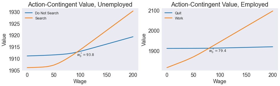
Compute and Print Critical Action Wages
def critical(db):
    wcrit = np.interp(0, db['value[active]'] - db['value[idle]'], db['wage'])
    vcrit = np.interp(wcrit, db['wage'], db['value[idle]'])
    return wcrit, vcrit

wcrit0, vcrit0 = critical(S.loc['unemployed'])
print(f'Critical Search Wage = {wcrit0:5.1f}')

wcrit1, vcrit1 = critical(S.loc['employed'])
print(f'Critical Quit Wage   = {wcrit1:5.1f}')
Critical Search Wage =  93.8
Critical Quit Wage   =  79.4
Plot Action-Contingent Value Function
vv = ['value[idle]','value[active]']
fig1, (ax0, ax1) = plt.subplots(1,2,figsize=[16,4])

# UNEMPLOYED
ax0.set(title='Action-Contingent Value, Unemployed', xlabel='Wage', ylabel='Value')
ax0.plot(S.loc['unemployed',vv])
ax0.annotate(f'$w^*_0 = {wcrit0:.1f}$', [wcrit0, vcrit0], fontsize=12, va='top')
ax0.legend(['Do Not Search', 'Search'], loc='upper left', fontsize="x-small")


# EMPLOYED
ax1.set(title='Action-Contingent Value, Employed', xlabel='Wage', ylabel='Value')
ax1.plot(S.loc['employed',vv])
ax1.annotate(f'$w^*_0 = {wcrit1:.1f}$', [wcrit1, vcrit1], fontsize=12, va='top')
ax1.legend(['Quit', 'Work'], loc='upper left', fontsize="x-small")
<matplotlib.legend.Legend at 0x1e145301a60>
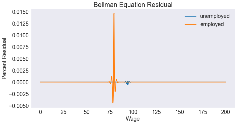
Plot Residual
S['resid2'] = 100 * (S['resid'] / S['value'])

fig2, ax = plt.subplots()

ax.set(title='Bellman Equation Residual',
       xlabel='Wage',
       ylabel='Percent Residual')
ax.plot(S.loc['unemployed','resid2'])
ax.plot(S.loc['employed','resid2'])
ax.legend(model.labels.i)
<matplotlib.legend.Legend at 0x1e140654250>
SIMULATION
Simulate Model
We simulate the model 10000 times for a time horizon \(T=40\), starting with an unemployed worker (\(i=0\)) at the long-term wage rate mean \(\bar{w}\). To be able to reproduce these results, we set the random seed at an arbitrary value of 945.
T = 40
nrep = 10000
sinit = np.full((1, nrep), wbar)
iinit = 0
data = model.simulate(T, sinit, iinit, seed=945)
data.head()
| time | _rep | i | wage | j* | |
|---|---|---|---|---|---|
| 0 | 0 | 0 | unemployed | 100.0 | active |
| 1 | 0 | 1 | unemployed | 100.0 | active |
| 2 | 0 | 2 | unemployed | 100.0 | active |
| 3 | 0 | 3 | unemployed | 100.0 | active |
| 4 | 0 | 4 | unemployed | 100.0 | active |
Print Ergodic Moments
ff = '\t{:12s} = {:5.2f}'

print('\nErgodic Means')
print(ff.format('Wage', data['wage'].mean()))
print(ff.format('Employment', (data['i'] == 'employed').mean()))
print('\nErgodic Standard Deviations')
print(ff.format('Wage',data['wage'].std()))
print(ff.format('Employment', (data['i'] == 'employed').std()))
Ergodic Means
	Wage         = 100.02
	Employment   =  0.58

Ergodic Standard Deviations
	Wage         =  5.37
	Employment   =  0.49
ergodic = pd.DataFrame({
    'Ergodic Means' : [data['wage'].mean(), (data['i'] == 'employed').mean()],
    'Ergodic Standard Deviations': [data['wage'].std(), (data['i'] == 'employed').std()]},
    index=['Wage', 'Employment'])

ergodic.round(2)
| Ergodic Means | Ergodic Standard Deviations | |
|---|---|---|
| Wage | 100.02 | 5.37 |
| Employment | 0.58 | 0.49 |
Plot Expected Discrete State Path
data.head()
| time | _rep | i | wage | j* | |
|---|---|---|---|---|---|
| 0 | 0 | 0 | unemployed | 100.0 | active |
| 1 | 0 | 1 | unemployed | 100.0 | active |
| 2 | 0 | 2 | unemployed | 100.0 | active |
| 3 | 0 | 3 | unemployed | 100.0 | active |
| 4 | 0 | 4 | unemployed | 100.0 | active |
data['ii'] = data['i'] == 'employed'
probability_of_employment = data[['ii','time']].groupby('time').mean()

fig3, ax = plt.subplots()
ax.set(title='Probability of Employment', xlabel='Period', ylabel='Probability')
ax.plot(probability_of_employment)
[<matplotlib.lines.Line2D at 0x1e14565f2b0>]

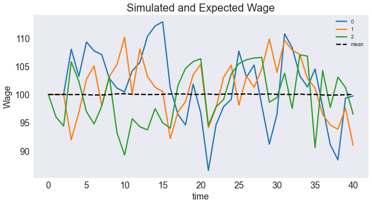
Plot Simulated and Expected Continuous State Path
subdata = data.query('_rep < 3').pivot("time", "_rep" ,'wage')

fig4, ax = plt.subplots()

ax.set(title='Simulated and Expected Wage', xlabel='Period', ylabel='Wage')
subdata.plot(ax=ax)
ax.plot(data[['time','wage']].groupby('time').mean(),'k--',label='mean')
ax.legend(fontsize='xx-small')
<matplotlib.legend.Legend at 0x1e1456e97f0>