Monte Carlo Simulation of Time Series
Contents
Monte Carlo Simulation of Time Series
Randall Romero Aguilar, PhD
This demo is based on the original Matlab demo accompanying the Computational Economics and Finance 2001 textbook by Mario Miranda and Paul Fackler.
Original (Matlab) CompEcon file: demqua10.m
Running this file requires the Python version of CompEcon. This can be installed with pip by running
!pip install compecon --upgrade
Last updated: 2022-Oct-23
About
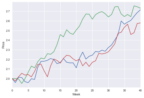
Simulate time series using Monte Carlo Method.
A commodity price is governed by weekly price movements
\[\begin{equation*}
\log(p_{t+1}) = \log(p_t) + \tilde \epsilon_t
\end{equation*}\]
where the \(\tilde \epsilon_t\) are i.i.d. normal with mean \(\mu=0.005\) and standard deviation \(\sigma=0.02\).
To simulate three time series of T=40 weekly price changes, starting from a price of 2, execute the script
Initial tasks
import numpy as np
from scipy.stats import norm
import matplotlib.pyplot as plt
plt.style.use('seaborn')
Simulation
m, T = 3, 40
mu, sigma = 0.005, 0.02
e = norm.rvs(mu,sigma,size=[T,m])
logp = np.zeros([T+1,m])
logp[0] = np.log(2)
for t in range(T):
    logp[t+1] = logp[t] + e[t]
Make figure
fig, ax = plt.subplots()
ax.set(xlabel='Week', ylabel='Price', xlim=[0,T])
ax.plot(np.exp(logp));