Linear-Quadratic Model
Contents
Linear-Quadratic Model
Randall Romero Aguilar, PhD
This demo is based on the original Matlab demo accompanying the Computational Economics and Finance 2001 textbook by Mario Miranda and Paul Fackler.
Original (Matlab) CompEcon file: demdp18.m
Running this file requires the Python version of CompEcon. This can be installed with pip by running
!pip install compecon --upgrade
Last updated: 2022-Oct-23
About
Simple Linear-Quadratic control example. Illustrates use of lqsolve.
States
s generic state of dimension ds=3
Actions
x generic action of dimension dx=2
import numpy as np
import matplotlib.pyplot as plt
from compecon import LQmodel, nodeunif
from mpl_toolkits.mplot3d import Axes3D
from matplotlib import cm
One-Dimensional Problem
# Input Model Parameters
F0  =  0.0
Fs  = -1.0
Fx  = -0.0
Fss = -1.0
Fsx =  0.0
Fxx = -0.1
G0  =  0.5
Gs  = -0.2
Gx  =  0.5
delta = 0.9
Solve model using LQmodel
model = LQmodel(F0,Fs,Fx,Fss,Fsx,Fxx,G0,Gs,Gx,delta)
model.steady
{'s': array([[-0.4528]]),
 'x': array([[-2.0867]]),
 'p': array([[-0.4637]]),
 'v': array([[1.3257]])}
sstar, xstar, pstar, vstar = model.steady_state
Plot results
n, smin, smax = 100, -5, 5
s = np.linspace(smin, smax, n)
S = model.solution(s)
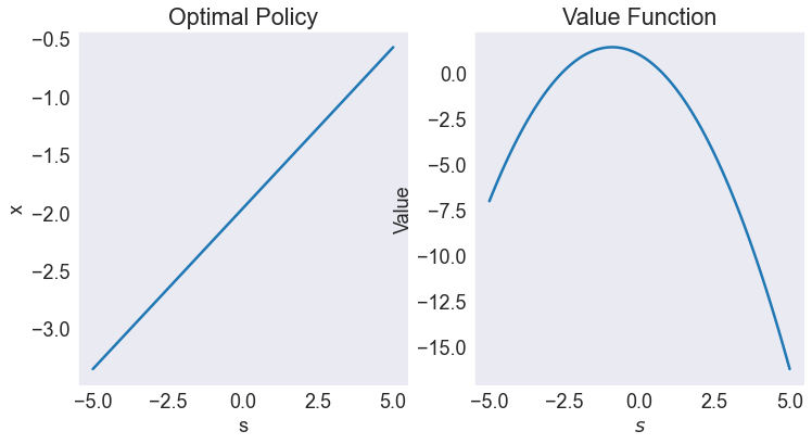
Optimal policy and value function
fig, axs = plt.subplots(1, 2)
S['x'].plot(ax=axs[0])
axs[0].set(title='Optimal Policy', xlabel='s', ylabel='x')

S['value'].plot(ax=axs[1])
axs[1].set(title='Value Function', xlabel='$s$', ylabel='Value');
Higher Dimensional Problem
F0  = 3
Fs  = [1, 0]
Fx  = [1, 1]
Fss = [[-7, -2],[-2, -8]]
Fsx = [[0, 0], [0, 1]]
Fxx = [[-2, 0], [0, -2]]
G0  = [[1], [1]]
Gs  = [[-1, 1],[1, 0]]
Gx  = [[-1, -1],[2, 3]]
delta = 0.95
model2 = LQmodel(F0,Fs,Fx,Fss,Fsx,Fxx,G0,Gs,Gx,delta)
n = [8,8]
ss = nodeunif(n,-1,1)
S2 = model2.solution(ss)
def plot3d(y):
    s0 = S2['s0'].values.reshape(n)
    s1 = S2['s1'].values.reshape(n)
    z = S2[y].values.reshape(n)

    fig = plt.figure(figsize=[12, 6])
    ax = fig.add_subplot(1, 1, 1, projection='3d')
    ax.plot_surface(s0, s1, z, rstride=1, cstride=1, cmap=cm.coolwarm,
                linewidth=0, antialiased=False)
    ax.set_xlabel('$s_0$')
    ax.set_ylabel('$s_1$')
    ax.set_zlabel(y)
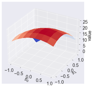
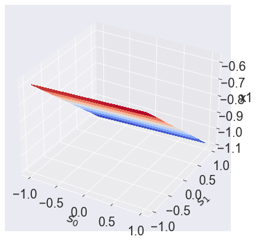
Value function
plot3d('value')
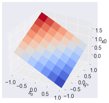
Optimal policy
plot3d('x0')
plot3d('x1')
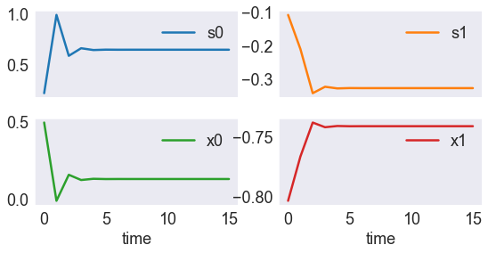
Simulations
sini = model2.steady['s']/3

data = model2.simulate(16,sini)
data.set_index('time', inplace=True)

data.plot(subplots=True,layout=(2,2), figsize=[9,4])
print(model2.steady['s'])
print(model2.steady['x'])
[[ 0.6436]
 [-0.3275]]
[[ 0.1272]
 [-0.7418]]