Deterministic Nonrenewable Resource Model
Contents
Deterministic Nonrenewable Resource Model
Randall Romero Aguilar, PhD
This demo is based on the original Matlab demo accompanying the Computational Economics and Finance 2001 textbook by Mario Miranda and Paul Fackler.
Original (Matlab) CompEcon file: demdoc03.m
Running this file requires the Python version of CompEcon. This can be installed with pip by running
!pip install compecon --upgrade
Last updated: 2021-Oct-01
About
Welfare maximizing social planner must decide the rate at which a nonrenewable resource should be harvested.
State
s resource stock
Control
q harvest rate
Parameters
κ harvest unit cost scale factor
γ harvest unit cost elasticity
η inverse elasticity of demand
𝜌 continuous discount rate
Preliminary tasks
Import relevant packages
import pandas as pd
import matplotlib.pyplot as plt
from compecon import BasisChebyshev, OCmodel
Model parameters
κ = 10     # harvest unit cost scale factor
γ = 1      # harvest unit cost elasticity
η = 1.5    # inverse elasticity of demand
𝜌 = 0.05   # continuous discount rate
Approximation structure
n = 20          # number of basis functions
smin = 0.1        # minimum state
smax = 1.0        # maximum state
basis = BasisChebyshev(n, smin, smax, labels=['q'])  # basis functions
Solve HJB equation by collocation
def control(s, Vs, κ, γ, η, 𝜌):
    k = κ * s**(-γ)
    return (Vs + k)**(-1/η)

def reward(s, q, κ, γ, η, 𝜌):
    u = (1/(1-η)) * q **(1-η)
    k = κ * s**(-γ)
    return u - k*q

def transition(s, q, κ, γ, η, 𝜌):
    return  -q

model = OCmodel(basis, control, reward, transition, rho=𝜌, params=[κ, γ, η, 𝜌])
data = model.solve()
Solving optimal control model
iter change       time
------------------------------
   0       5.4e+02    0.0010
   1       1.2e+02    0.0020
   2       3.2e+01    0.0020
   3       9.2e+00    0.0030
   4       1.0e+00    0.0030
   5       7.2e-03    0.0030
   6       1.6e-06    0.0040
   7       4.5e-09    0.0040
Elapsed Time =    0.00 Seconds
Plots
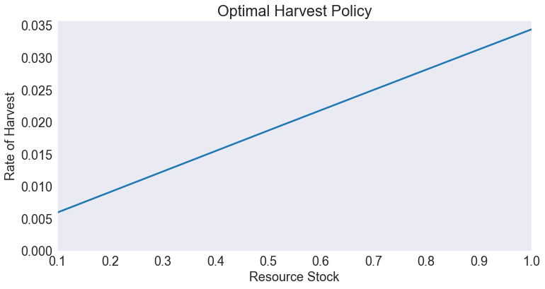
Optimal policy
fig, ax = plt.subplots()
data['control'].plot(ax=ax)
ax.set(title='Optimal Harvest Policy',
       xlabel='Resource Stock',
       ylabel='Rate of Harvest',
       xlim=[smin, smax])
ax.set_ylim(bottom=0)
(0.0, 0.03578278411627879)
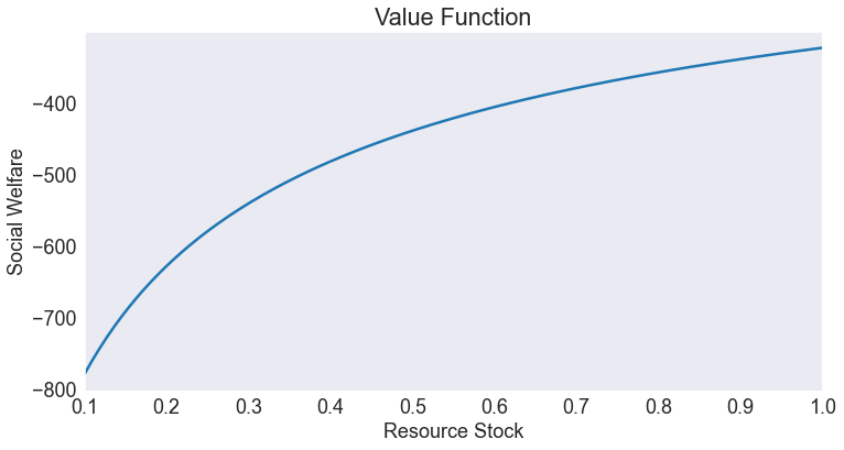
Value function
fig, ax = plt.subplots()
data['value'].plot(ax=ax)
ax.set(title='Value Function',
       xlabel='Resource Stock',
       ylabel='Social Welfare',
       xlim=[smin, smax])
[Text(0.5, 1.0, 'Value Function'),
 Text(0.5, 0, 'Resource Stock'),
 Text(0, 0.5, 'Social Welfare'),
 (0.1, 1.0)]
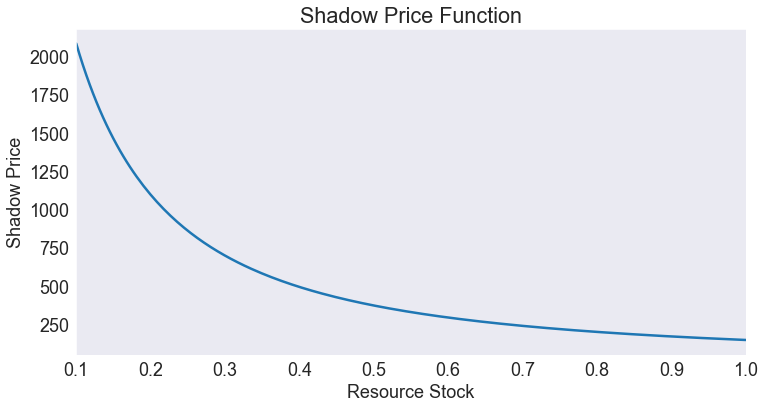
Shadow price
data['shadow'] = model.Value(data.index, 1)

fig, ax = plt.subplots()
data['shadow'].plot(ax=ax)
ax.set(title='Shadow Price Function',
       xlabel='Resource Stock',
       ylabel='Shadow Price',
       xlim=[smin, smax])
[Text(0.5, 1.0, 'Shadow Price Function'),
 Text(0.5, 0, 'Resource Stock'),
 Text(0, 0.5, 'Shadow Price'),
 (0.1, 1.0)]
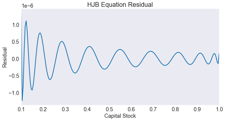
Residual
fig, ax = plt.subplots()
data['resid'].plot(ax=ax)
ax.set(title='HJB Equation Residual',
       xlabel='Capital Stock',
       ylabel='Residual',
       xlim=[smin, smax]);
Simulate the model
Initial state and time horizon
s0 = smax  # initial capital stock
T  = 40    # time horizon
Simulation and plot
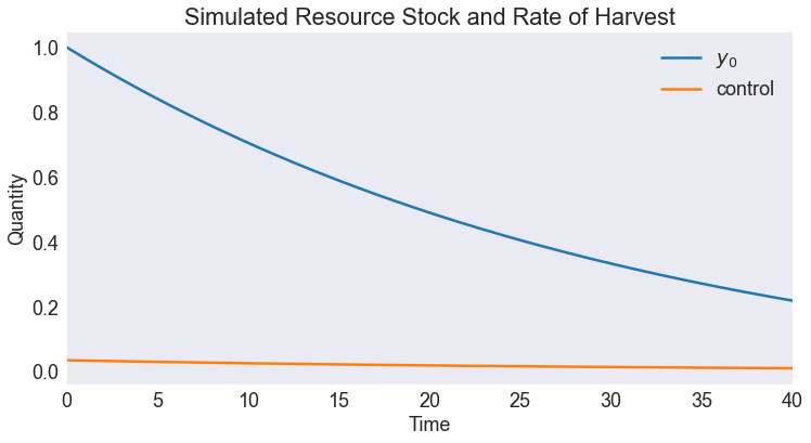
fig, ax = plt.subplots()
model.simulate([s0], T).plot(ax=ax)
ax.set(title='Simulated Resource Stock and Rate of Harvest',
       xlabel='Time',
       ylabel='Quantity',
       xlim=[0, T])

#ax.legend([]);
PARAMETER xnames NO LONGER VALID. SET labels= AT OBJECT CREATION
[Text(0.5, 1.0, 'Simulated Resource Stock and Rate of Harvest'),
 Text(0.5, 0, 'Time'),
 Text(0, 0.5, 'Quantity'),
 (0.0, 40.0)]