Industry Entry-Exit Model

Industry Entry-Exit Model¶

Randall Romero Aguilar, PhD

This demo is based on the original Matlab demo accompanying the Computational Economics and Finance 2001 textbook by Mario Miranda and Paul Fackler.

Original (Matlab) CompEcon file: demdp03.m

Running this file requires the Python version of CompEcon. This can be installed with pip by running

!pip install compecon --upgrade

Last updated: 2022-Oct-10

About¶

A firm operates in an uncertain profit environment. At the beginning of each period, the firm observes its potential short-run operating profit over the coming period \(\pi\), which may be negative, and decides whether to operate, making a short-run profit \(\pi\), or not operate, making a short-run profit \(0\). Although the firm faces no fixed costs, it incurs a shutdown cost \(K_0\) when it closes and a start-up cost \(K_1\) when it reopens. The short-run profit \(\pi\) is an exogenous continuous-valued Markov process

(16)¶\[\begin{equation} \pi_{t+1} = h(\pi_t, \epsilon_{t+1}) \end{equation}\]

What is the optimal entry-exit policy? In particular, how low must the short-run profit be for an operating firm to close, and how high must the short-run profit be for nonoperating firm to reopen?

This is an infinite horizon, stochastic model with time \(t\) measured in years. The state variables

(17)¶\[\begin{align} \pi &\in (−\infty,\infty)\\ d &\in \{0, 1\} \end{align}\]

are the current short-run profit, a continuous variable, and the operational status of the firm, a binary variable that equals 1 if the firm is operating and 0 if the firm is not operating. The choice variable

(18)¶\[\begin{equation} j \in \{0, 1\} \end{equation}\]

is the operating decision for the coming year, a binary variable that equals 1 if the firm operates and 0 if does not operate. The state transition function is

(19)¶\[\begin{equation} g(\pi, d, j, \epsilon) = h(\pi, \epsilon), j) \end{equation}\]

The reward function is

(20)¶\[\begin{equation} f(\pi, d, j) = \pi j − K_1(1 − d)j − K_0 d(1 − j) \end{equation}\]

The value of the firm, given that the current short-run profit is \(\pi\) and the firm’s operational status is \(d\), satisfies the Bellman equation

(21)¶\[\begin{equation} V(\pi,d) = \max_{j=0,1}\left\{\pi j − K_1(1−d)j − K_0d(1−j) + \delta E_\epsilon V\left(h(\pi,\epsilon),j\right)\right\} \end{equation}\]

import numpy as np
import pandas as pd
import matplotlib.pyplot as plt
from compecon import BasisSpline, DPmodel,qnwnorm

The reward function¶

The reward function is

(22)¶\[\begin{equation} f(\pi, d, j) = \pi j − K_1(1 − d)j − K_0 d(1 − j) \end{equation}\]

where the exit cost is \(K_0=0\) and the entry cost is \(K_1=10\).

K0     = 0.0
K1     = 10

def profit(p, x, d, j):
    return p * j - K1 * (1 - d) * j - K0 * d * (1 - j)

The transition function¶

Assuming that the short-run profit \(\pi\) is an exogenous Markov process

(23)¶\[\begin{equation} \pi_{t+1} = g(\pi_t,\epsilon_{t+1}) = \bar{\pi} + \gamma(\pi_t − \bar{\pi}) + \epsilon_{t+1} \end{equation}\]

where \(\bar{\pi}=1.0\) and \(\gamma=0.7\).

pbar   = 1.0
gamma  = 0.7

def transition(p, x, d, j, in_, e):
    return pbar + gamma * (p - pbar) + e

In the transition function \(\epsilon_t\) is an i.i.d. normal(0, \(σ^2\)), with \(\sigma=1\). We discretize this distribution by using a discrete distribution, matching the first 10 moments of the normal distribution.

m = 5  # number of profit shocks
sigma  = 1.0
[e,w] = qnwnorm(m,0,sigma **2)

The collocation method calls for the analyst to select \(n\) basis functions \(\varphi_j\) and \(n\) collocation nodes \((\pi_i,d_i)\), and form the value function approximant \(V(\pi,d) \approx \sum_{j=1}^{n} c_j\varphi_j(\pi,d)\) whose coefficients \(c_j\) solve the collocation equation

(24)¶\[\begin{equation} \sum_{j=1}^{n} c_j\varphi_j(\pi_i,d_i) = \max_{x\in\{0,1\}}\left\{\pi_i x − K_1(1−d_i)x − K_0 d_i(1−x) + \delta\sum_{k=1}^{m}\sum_{j=1}^{n}w_k c_j \varphi_j(\hat{\pi}_{ik},x)\right\} \end{equation}\]

where \(\hat\pi_{ik}=g(\pi_i,\epsilon_k)\) and where \(\epsilon_k\) and \(w_k\) represent quadrature nodes and weights for the normal shock.

For the approximation, we use a cubic spline basis with \(n=250\) nodes between \(p_\text{min}=-20\) and \(p_\text{max}=20\).

n = 250
pmin = -20
pmax =  20
basis = BasisSpline(n, pmin, pmax, labels=['profit'])
print(basis)

A 1-dimension Cubic spline basis:  using 250 Canonical nodes and 250 polynomials
___________________________________________________________________________
	profit: 250 nodes in [-20.00,  20.00]

===========================================================================
WARNING! Class Basis is still work in progress

Discrete states and discrete actions are

dstates = ['idle', 'active']
dactions = ['close', 'open']

The Bellman equation is represeted by a DPmodel object, where we assume a discount factor of \(\delta=0.9\). Notice that the discrete state transition is deterministic, with transition matrix

(25)¶\[\begin{equation} h=\begin{bmatrix}0&0\\1&1\end{bmatrix} \end{equation}\]

model = DPmodel(basis,
                profit, transition,
                i=dstates,
                j=dactions,
                discount=0.9, e=e, w=w,
                h=[[0, 0], [1, 1]])

SOLUTION¶

To solve the model, we simply call the solve method on the model object.

S = model.solve(show=True)
S.head()

Solving infinite-horizon model collocation equation by Newton's method
iter change       time    
------------------------------
   0       6.0e+01    0.0625
   1       3.2e+01    0.1099

   2       2.9e+00    0.1725

   3       4.3e-01    0.2350
   4       4.9e-14    0.2975
Elapsed Time =    0.30 Seconds

		profit	i	value	resid	j*	value[close]	value[open]
	profit
idle	-20.000000	-20.000000	0	0.894342	-1.110223e-16	close	0.894342	-29.105658
	-19.983994	-19.983994	0	0.894542	-5.251344e-11	close	0.894542	-29.089452
	-19.967987	-19.967987	0	0.894743	-5.991030e-11	close	0.894743	-29.073245
	-19.951981	-19.951981	0	0.894943	-2.191858e-11	close	0.894943	-29.057038
	-19.935974	-19.935974	0	0.895144	4.235901e-11	close	0.895144	-29.040830

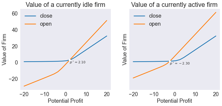
Plot Action-Contingent Value Functions¶

fig1,axs = plt.subplots(1,2,sharey=True, figsize=[12,5])

msgs = ['Profit Entry', 'Profit Exit']

for ax, state in zip(axs, dstates):
    subdata = S.loc[state, ['value[close]', 'value[open]']]
    ax.plot(subdata)
    ax.set(title= f"Value of a currently {state} firm",
           xlabel='Potential Profit',
           ylabel='Value of Firm')
    
    ax.legend(dactions)
    
    subdata['v.diff'] = subdata['value[open]'] - subdata['value[close]']
    pcrit = np.interp(0, subdata['v.diff'], subdata.index)
    vcrit  = np.interp(pcrit, subdata.index, subdata['value[close]'])
    
    ax.plot(pcrit, vcrit, 'wo')
    ax.annotate(f'$p^* = {pcrit:.2f}$', [pcrit, vcrit], fontsize=11, va='top')
    

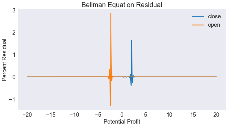
../../_images/03 Industry Entry-Exit Model_18_0.png

Plot Residual¶

We normalize the residuals as percentage of the value function. Notice the spikes at the “Profit entry” and “Profit exit” points.

S['resid2'] = 100 * (S.resid / S.value)

fig2, ax = plt.subplots()

ax.plot(S['resid2'].unstack(level=0))
ax.set(title='Bellman Equation Residual',
       xlabel='Potential Profit',
       ylabel='Percent Residual')
       
ax.legend(dactions);

../../_images/03 Industry Entry-Exit Model_20_0.png

SIMULATION¶

We simulate the model 50000 times for a time horizon \(T=50\), starting with an operating firm (\(d=1\)) at the long-term profit mean \(\bar{\pi}\). To be able to reproduce these results, we set the random seed at an arbitrary value of 945.

T = 50
nrep = 50000
p0 = np.tile(pbar, (1, nrep))
d0 = 1
data = model.simulate(T, p0, d0, seed=945)

Print Ergodic Moments¶

ergodic = pd.DataFrame({
    'Ergodic Means' : [data['profit'].mean(), (data['i'] == 'active').mean()],
    'Ergodic Standard Deviations': [data['profit'].std(), (data['i'] == 'active').std()]},
    index=['Profit Contribution', 'Activity'])

ergodic.round(2)

	Ergodic Means	Ergodic Standard Deviations
Profit Contribution	1.00	1.37
Activity	0.94	0.24

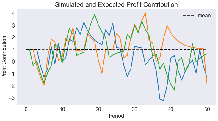
Plot Simulated and Expected Continuous State Path¶

subdata = data.query("_rep < 3").set_index(["time", "_rep"]).unstack()

fig3, ax = plt.subplots()

ax.plot(subdata["profit"])
ax.set(title='Simulated and Expected Profit Contribution', 
       xlabel='Period',
       ylabel='Profit Contribution')

ax.plot(data[['time','profit']].groupby('time').mean(),'k--',label='mean')
ax.legend();

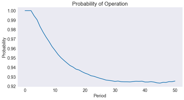
../../_images/03 Industry Entry-Exit Model_27_0.png

Plot Expected Discrete State Path¶

data['ii'] = data['i'] == 'active'
probability_of_active = data[['time','ii']].groupby('time').mean()

fig4, ax = plt.subplots()

ax.plot(probability_of_active)
ax.set(title='Probability of Operation', 
       xlabel='Period', 
       ylabel='Probability');

../../_images/03 Industry Entry-Exit Model_29_0.png

Asset Replacement Model

Job Search Model

A Python Implementation of CompEcon