American Put Option Pricing Model
Contents
American Put Option Pricing Model
Randall Romero Aguilar, PhD
This demo is based on the original Matlab demo accompanying the Computational Economics and Finance 2001 textbook by Mario Miranda and Paul Fackler.
Original (Matlab) CompEcon file: demdp05.m
Running this file requires the Python version of CompEcon. This can be installed with pip by running
!pip install compecon --upgrade
Last updated: 2022-Oct-23
About
An American put option gives the holder the right, but not the obligation, to sell a specified quantity of a commodity at a specified strike price \(K\) on or before a specified expiration period \(T\). In the discrete time, continuous state Black-Scholes option pricing model, the price of the commodity follows an exogenous continuous-valued Markov process
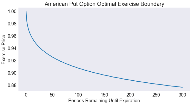
What is the value of an American put option in period \(t\) if the commodity price is \(P\)? At what critical price is it optimal to exercise the put option, and how does this critical price vary over time?
This is a finite horizon, stochastic model with time \(t\) measured in periods. The state variables
are the current commodity price, a continuous variable, and the exercise status of the option, a discrete variable that equals 1 if the option has been exercised previously and equals 0 otherwise. The action variable
is the exercise decision, a discrete variable that equals 1 if the option is exercised and equals 0 otherwise. The state transition function is
The reward function is
The value of an unexercised option in period \(t\), given that the commodity price is \(P\), satisfies the Bellman equation
subject to the terminal condition \(V_{T+1}(P,1) = 0\). The value of a previously exercised option is zero, regardless of the price of the commodity; that is, \(V_t(P,1) = 0\) for all \(P\) and \(t\).
Preliminary tasks
import numpy as np
import matplotlib.pyplot as plt
from compecon import BasisSpline, NLP, qnwnorm
FORMULATION
In what follows, we are going to solve the problem in term of the log-price, defining \(p\equiv\log(P)\). We assume that log-price of the commodity follows a random walk:
where \(\epsilon\) is a normal \((\mu, \sigma^2)\) shock. We discretize this distribution by using qnwnorm, assuming that \(\mu=0.0001,\quad\sigma=0.008\) and setting up \(m=15\) nodes.
μ, σ    = 0.0001, 0.0080
m = 15
[e,w] = qnwnorm(m,μ,σ**2)
We are going to compute the critical exercise price in terms of the time to expiration, up to an horizon of \(T=300\) periods. First we allocate memory for the critical prices:
T = 300
pcrit = np.empty(T + 1)
The critical exercise price is the price at which the value of exercising the option \(K-\exp(p)\) equals the discounted expected value of keeping the option one more period \(\delta E_\epsilon V(p + \epsilon)\). To find it, we set it as a nonlinear rootfinding problem by using the NLP class; here we assume that the option strike price is \(K=1\) and that the discount factor is \(\delta=0.9998\)
K = 1.0
δ = 0.9998
f = NLP(lambda p: K - np.exp(p) - δ * Value(p))
Notice that we have not defined the Value(p) function yet. This function is unknown, so we are going to approximate it with a cubic spline, setting 500 nodes between -1 and 1. Since the basis is expressed in terms of log-prices, this interval corresponds to prices between 0.3679 and 2.7183.
n = 500
pmin  = -1 # minimum log price
pmax  =  1 # maximum log price
Value = BasisSpline(n, pmin, pmax,
                    labels=['logprice'], l=['value'])
print(Value)
A 1-dimension Cubic spline basis:  using 500 Canonical nodes and 500 polynomials
___________________________________________________________________________
	logprice: 500 nodes in [ -1.00,   1.00]

===========================================================================
WARNING! Class Basis is still work in progress
In the last expression, by passing the option l with a one-element list we are telling the BasisSpline class that we a single function named “value”. On creation, the function will be set by default to \(V(p)=0\) for all values of \(p\), which conveniently corresponds to the terminal condition of this problem.
Finding the critical exercise prices
We are going to find the prices recursively, starting form a option in the expiration date. Notice that the solution to this problem is trivial: since next-period value is zero, the exercise price is \(K\). Either way, we can find it numerically by calling the zero method on the f object.
pcrit[0] = f.zero(0.0)
Next, for each possible price shock, we compute next period log-price by adding the shock to current log-prices (the nodes of the Value object). Then, we use each next-period price to compute the expected value of an option with one-period to maturity (save the values in v). We update the value function to reflect the new time-to-maturity and use broyden to solve for the critical value. We repeat this procedure until we reach the \(T=300\) horizon.
for t in range(T):
    v = np.zeros((1, n))
    for k in range(m):
        pnext = Value.nodes + e[k]
        v += w[k] * np.maximum(K - np.exp(pnext), δ * Value(pnext))

    Value[:] = v
    pcrit[t + 1] = f.broyden(pcrit[t])
Print Critical Exercise Price 300 Periods to Expiration
print('Critical Price = %5.2f' % np.exp(pcrit[-1]))
Critical Price = 0.88
Plot Critical Exercise Prices
fig1, ax = plt.subplots()

ax.set(title='American Put Option Optimal Exercise Boundary',
       xlabel='Periods Remaining Until Expiration',
       ylabel='Exercise Price')

ax.plot(np.exp(pcrit))
[<matplotlib.lines.Line2D at 0x2737cf0cb20>]

