Ito Processes
Contents
Ito Processes
Randall Romero Aguilar, PhD
This demo is based on the original Matlab demo accompanying the Computational Economics and Finance 2001 textbook by Mario Miranda and Paul Fackler.
Original (Matlab) CompEcon file: demsoc00.m
Running this file requires the Python version of CompEcon. This can be installed with pip by running
!pip install compecon --upgrade
Last updated: 2021-Oct-01
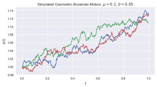
Simulate geometric Brownian motion
import numpy as np
import matplotlib.pyplot as plt
plt.style.use('seaborn')
Model Parameters
T = 1
n = 365
t = np.linspace(0, T, n)
h = t[1] - t[0]

𝜇 = 0.1
𝜎 = 0.05
Simulate
m = 3
z = np.random.randn(n,m)
s = np.zeros((n,m))
s[0] = 1
for i in range(n-1):
    s[i+1] = s[i] + 𝜇*s[i]*h + 𝜎*s[i]*np.sqrt(h)*z[i]
Plot
fig, ax = plt.subplots(figsize=[8,4])
ax.plot(t,s)
ax.set(xlabel='$t$',
       ylabel='$s(t)$',
       title='Simulated Geometric Brownian Motion, $\mu=0.1$, $\sigma=0.05$');
#fig.savefig('demsoc00-01.pdf', bbox_inches='tight')