Stochastic Optimal Economic Growth Model
Contents
Stochastic Optimal Economic Growth Model
Randall Romero Aguilar, PhD
This demo is based on the original Matlab demo accompanying the Computational Economics and Finance 2001 textbook by Mario Miranda and Paul Fackler.
Original (Matlab) CompEcon file: demdp07.m
Running this file requires the Python version of CompEcon. This can be installed with pip by running
!pip install compecon --upgrade
Last updated: 2022-Oct-23
About
Welfare maximizing social planner must decide how much society should consume and invest. Unlike the deterministic model, this model allows arbitrary constant relative risk aversion, capital depreciation, and stochastic production shocks. It lacks a known closed-form solution.
States
s stock of wealth
Actions
k capital investment
Parameters
ɑ relative risk aversion
β capital production elasticity
ɣ capital survival rate
σ production shock volatility
δ discount factor
import numpy as np
import matplotlib.pyplot as plt
from compecon import BasisChebyshev, DPmodel, DPoptions, qnwlogn
import seaborn as sns
import pandas as pd
Model parameters
α, β, γ, σ, δ = 0.2, 0.5, 0.9, 0.1, 0.9
Analytic results
The deterministic steady-state values for this model are
kstar = ((1 - δ*γ)/(δ*β))**(1/(β-1))  # steady-state capital investment

sstar = γ*kstar + kstar**β            # steady-state wealth
Numeric results
State space
The state variable is s=”Wealth”, which we restrict to \(s\in[5, 10]\).
Here, we represent it with a Chebyshev basis, with \(n=10\) nodes.
n, smin, smax = 10, 5, 10
basis = BasisChebyshev(n, smin, smax, labels=['Wealth'])
Continuous state shock distribution
m = 5
e, w = qnwlogn(m, -σ**2/2,σ**2)
Action space
The choice variable k=”Investment” must be nonnegative.
def bounds(s, i=None, j=None):
    return np.zeros_like(s), 0.99*s
Reward function
The reward function is the utility of consumption=\(s-k\).
def reward(s, k, i=None, j=None):
    sk = s - k
    u = sk**(1-α) / (1-α)
    ux= -sk **(-α)
    uxx = -α * sk**(-1-α)
    return u, ux, uxx
State transition function
Next period, wealth will be equal to production from available initial capital \(k\), that is \(s' = k^\beta\)
def transition(s, k, i=None, j=None, in_=None, e=None):
    g = γ * k  + e * k**β
    gx = γ  + β*e * k**(β-1)
    gxx = β*(β-1)*e * k**(β-2)
    return g, gx, gxx
Model structure
The value of wealth \(s\) satisfies the Bellman equation
To solve and simulate this model,use the CompEcon class DPmodel
growth_model = DPmodel(basis, reward, transition, bounds,e=e,w=w,
                       x=['Investment'],
                       discount=δ )
Solving the model
Solving the growth model by collocation.
S = growth_model.solve()
Solving infinite-horizon model collocation equation by Newton's method
iter change       time
------------------------------
   0       8.2e+00    0.0000
   1       9.6e+00    0.0781
   2       2.2e+00    0.1250
   3       3.8e-02    0.1718
   4       7.0e-06    0.2030
   5       7.1e-15    0.2191
Elapsed Time =    0.22 Seconds
DPmodel.solve returns a pandas DataFrame with the following data:
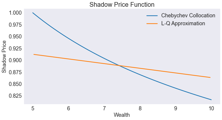
We are also interested in the shadow price of wealth (the first derivative of the value function).
To analyze the dynamics of the model, it also helps to compute the optimal change of wealth.
S['shadow price'] = growth_model.Value(S['Wealth'],1)
S['D.Wealth'] = transition(S['Wealth'], S['Investment'],e=1)[0] - S['Wealth']
S.head()
| Wealth | value | resid | Investment | shadow price | D.Wealth | |
|---|---|---|---|---|---|---|
| Wealth | ||||||
| 5.000000 | 5.000000 | 17.793592 | 4.324104e-09 | 3.997670 | 0.999535 | 0.597321 |
| 5.050505 | 5.050505 | 17.843995 | -1.837417e-09 | 4.032514 | 0.996440 | 0.586869 |
| 5.101010 | 5.101010 | 17.894243 | -4.078490e-09 | 4.067300 | 0.993391 | 0.576314 |
| 5.151515 | 5.151515 | 17.944339 | -3.954334e-09 | 4.102028 | 0.990386 | 0.565657 |
| 5.202020 | 5.202020 | 17.994283 | -2.583509e-09 | 4.136700 | 0.987425 | 0.554898 |
Solving the model by Linear-Quadratic Approximation
The DPmodel.lqapprox solves the linear-quadratic approximation, in this case arround the steady-state. It returns a LQmodel which works similar to the DPmodel object. We also compute the shadow price and the approximation error to compare these results to the collocation results.
growth_lq = growth_model.lqapprox(sstar, kstar)
L = growth_lq.solution(basis.nodes)
L['shadow price'] = L['value_Wealth']
L['D.Wealth'] = L['Wealth_next']- L['Wealth']
L.head()
| Wealth | Investment | value | value_Wealth | Wealth_next | shadow price | D.Wealth | |
|---|---|---|---|---|---|---|---|
| Wealth | |||||||
| 5.030779 | 5.030779 | 3.461913 | 17.923286 | 0.911808 | 5.030781 | 0.911808 | 1.397911e-06 |
| 5.272484 | 5.272484 | 3.679447 | 18.143387 | 0.909432 | 5.272485 | 0.909432 | 1.256542e-06 |
| 5.732233 | 5.732233 | 4.093221 | 18.560459 | 0.904912 | 5.732234 | 0.904912 | 9.876423e-07 |
| 6.365024 | 6.365024 | 4.662732 | 19.131111 | 0.898692 | 6.365024 | 0.898692 | 6.175332e-07 |
| 7.108914 | 7.108914 | 5.332233 | 19.796920 | 0.891380 | 7.108914 | 0.891380 | 1.824439e-07 |
Plotting the results
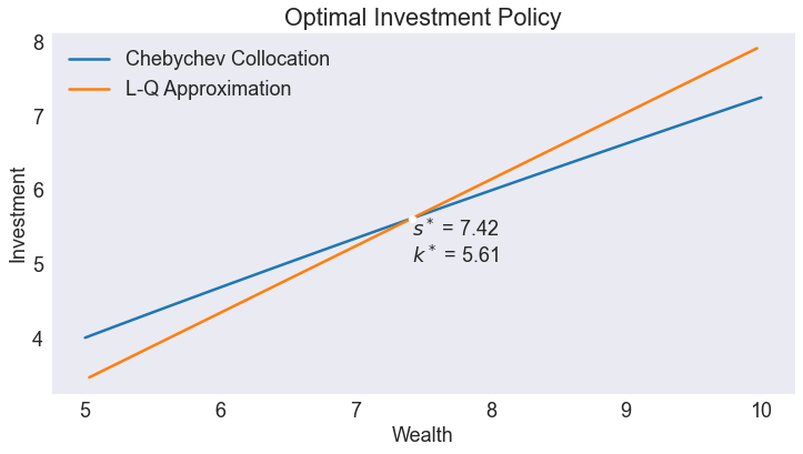
Optimal Policy
fig1, ax = plt.subplots()
ax.set(title='Optimal Investment Policy', xlabel='Wealth', ylabel='Investment')
ax.plot(S.Investment, label='Chebychev Collocation')
ax.plot(L.Investment, label='L-Q Approximation')

ax.plot(sstar, kstar,'wo')
ax.annotate(f"$s^*$ = {sstar:.2f}\n$k^*$ = {kstar:.2f}",[sstar, kstar],va='top')
ax.legend(loc= 'upper left');
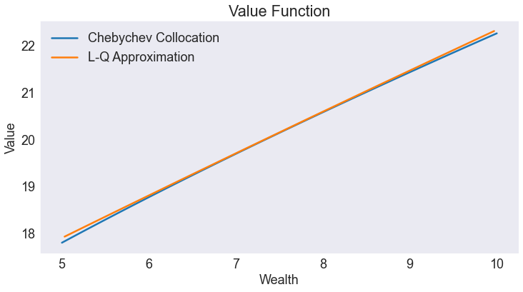
Value Function
fig2, ax = plt.subplots()
ax.set(title='Value Function', xlabel='Wealth', ylabel='Value')
ax.plot(S.value, label='Chebychev Collocation')
ax.plot(L.value, label='L-Q Approximation')
ax.legend(loc= 'upper left');
Shadow Price Function
fig3, ax = plt.subplots()
ax.set(title='Shadow Price Function', xlabel='Wealth', ylabel='Shadow Price')
ax.plot(S['shadow price'], label='Chebychev Collocation')
ax.plot(L['shadow price'], label='L-Q Approximation')
ax.legend(loc= 'upper right');
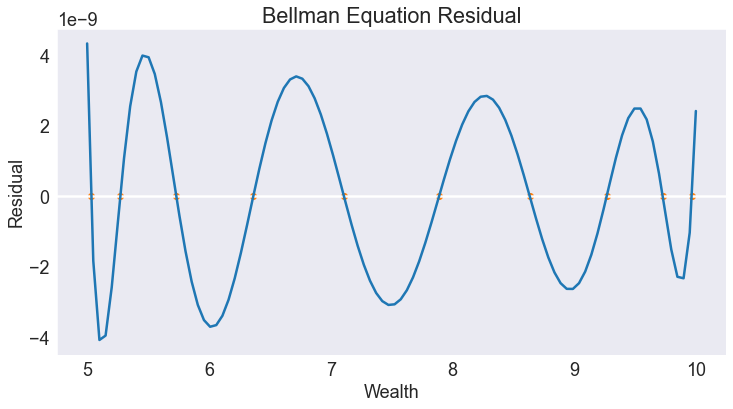
Chebychev Collocation Residual
fig4, ax = plt.subplots()
ax.set(title='Bellman Equation Residual', xlabel='Wealth', ylabel='Residual')
ax.axhline(0, color='w')
ax.plot(S[['resid']])
ax.scatter(basis.nodes[0], np.zeros_like(basis.nodes[0]), color='C1')
ax.ticklabel_format(style='sci', axis='y', scilimits=(-1,1))
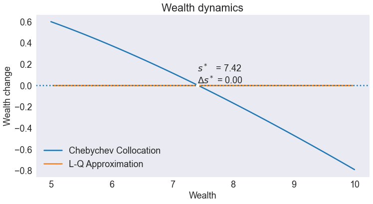
Wealth dynamics
Notice how the steady-state is stable in the Chebyshev collocation solution, but unstable in the linear-quadratic approximation. In particular, simulated paths of wealth in the L-Q approximation will converge to zero, unless the initial states is within a small neighborhood of the steady-state.
fig5, ax = plt.subplots()
ax.set(title='Wealth dynamics', xlabel='Wealth', ylabel='Wealth change')
ax.plot(S['D.Wealth'], label='Chebychev Collocation')
ax.plot(L['D.Wealth'], label='L-Q Approximation')
ax.axhline(0, linestyle=':')
ax.plot(sstar, 0, 'wo')
ax.annotate(f"$s^*$   = {sstar:.2f}\n$\Delta s^*$ = 0.00",[sstar, 0], va='bottom')
plt.legend(loc= 'lower left');
Simulating the model
We simulate 21 periods of the model starting from \(s=s_{\min}\)
T = 21
nrep = 50_000
data = growth_model.simulate(T, np.tile(smin,nrep))
Simulated State and Policy Paths
subdata = data.query('_rep < 100')
fig6, ax = plt.subplots()
ax.set(title='Simulated and Expected Wealth',
       xlabel='Period',
       ylabel='Wealth',
       xlim=[0, T + 0.5])

ax.plot(data[['time','Wealth']].groupby('time').mean())
ax.plot(subdata.pivot('time','_rep','Wealth'), lw=1, color='C0', alpha=0.2)
ax.annotate(f'steady-state wealth\n = {sstar:.2f}', [T, sstar-0.03], color='C0', va='top', ha='right')
Text(21, 7.386897506925211, 'steady-state wealth\n = 7.42')
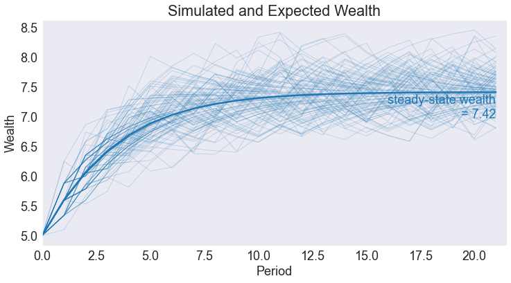
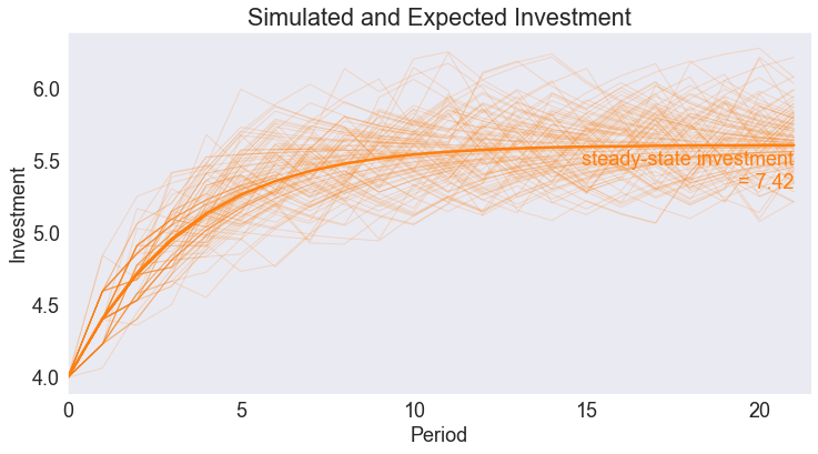
fig7, ax = plt.subplots()
ax.set(title='Simulated and Expected Investment',
       xlabel='Period',
       ylabel='Investment',
       xlim=[0, T + 0.5],
       xticks=range(0,T+1,5))

ax.plot(data[['time','Investment']].groupby('time').mean(), color='C1')
ax.plot(subdata.pivot('time','_rep','Investment'),lw=1, color='C1', alpha=0.2)

ax.annotate(f'steady-state investment\n = {sstar:.2f}', [T, kstar-0.03], color='C1', va='top', ha='right')
Text(21, 5.579418282548479, 'steady-state investment\n = 7.42')
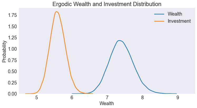
Ergodic Wealth Distribution
data.query("time == @T")
| time | _rep | Wealth | Investment | |
|---|---|---|---|---|
| 1050000 | 21 | 0 | 7.316155 | 5.544752 |
| 1050001 | 21 | 1 | 7.340926 | 5.560817 |
| 1050002 | 21 | 2 | 7.582651 | 5.717136 |
| 1050003 | 21 | 3 | 7.236199 | 5.492836 |
| 1050004 | 21 | 4 | 7.489982 | 5.657305 |
| ... | ... | ... | ... | ... |
| 1099995 | 21 | 49995 | 7.827284 | 5.874527 |
| 1099996 | 21 | 49996 | 7.302025 | 5.535583 |
| 1099997 | 21 | 49997 | 7.833176 | 5.878308 |
| 1099998 | 21 | 49998 | 7.309855 | 5.540664 |
| 1099999 | 21 | 49999 | 7.911989 | 5.928839 |
50000 rows × 4 columns
subdata = data.query("time == @T")[['Wealth','Investment']]
stats =pd.DataFrame({'Deterministic Steady-State': [sstar, kstar],
              'Ergodic Means': subdata.mean(),
              'Ergodic Standard Deviations': subdata.std()}).T
stats
| Wealth | Investment | |
|---|---|---|
| Deterministic Steady-State | 7.416898 | 5.609418 |
| Ergodic Means | 7.410732 | 5.605236 |
| Ergodic Standard Deviations | 0.339563 | 0.219709 |
fig8, ax = plt.subplots()

ax.set(title='Ergodic Wealth and Investment Distribution',
       xlabel='Wealth',
       ylabel='Probability',
       xlim=[4.5, 9.5])

sns.kdeplot(subdata['Wealth'], ax=ax, label='Wealth')
sns.kdeplot(subdata['Investment'], ax=ax, label='Investment')
ax.legend();