Change in Consumer Surplus
Contents
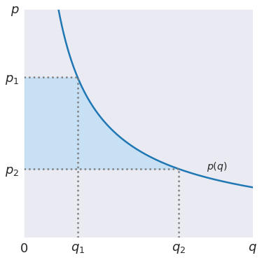
Change in Consumer Surplus
Randall Romero Aguilar, PhD
This demo is based on the original Matlab demo accompanying the Computational Economics and Finance 2001 textbook by Mario Miranda and Paul Fackler.
Original (Matlab) CompEcon file: demqua50.m
Running this file requires the Python version of CompEcon. This can be installed with pip by running
!pip install compecon --upgrade
Last updated: 2022-Oct-23
Initial tasks
from compecon import qnwlege
import numpy as np
import matplotlib.pyplot as plt
Define inverse demand curve
f = lambda p: 0.15*p**(-1.25)
p, w = qnwlege(11, 0.3, 0.7)
change = w.dot(f(p))
change
0.1547610245267632
Make figure
# Initiate figure
fig0, ax = plt.subplots()

# Set plotting parameters
n = 1001
qmin, qmax = 0, 1
pmin, pmax = 0, 1
p1, p2 = 0.7, 0.3

q1 = f(p1)
q2 = f(p2)

# Plot area under inverse demand curve
p = np.linspace(0,pmax, n)
q = f(p)

par = np.linspace(p2,p1, n)
ax.fill_betweenx(par, f(par), qmin, alpha=0.35, color='LightSkyBlue')

# Plot inverse demand curve
ax.plot(q,p)

# Annotate figure

ax.hlines([p1, p2], qmin, [q1, q2], linestyles=':', colors='gray')
ax.vlines([q1, q2], pmin, [p1, p2], linestyles=':', colors='gray')

ax.annotate('$p(q)$', [0.8,0.3], fontsize=14)

# To compute the change in consumer surplus `numerically'
[x,w] = qnwlege(15,p2,p1)
intn = w.T * f(x)

# To compute the change in consumer surplus `analytically'
F = lambda p: (0.15/(1-1.25))*p**(1-1.25)
inta = F(p1)-F(p2)

ax.set_aspect('equal')
ax.set(xlim=[qmin, qmax], xticks=[qmin,q1,q2,qmax], xticklabels=[r'$0$', r'$q_1$',r'$q_2$',r'$q$'],
       ylim=[pmin, pmax], yticks= [p1, p2, pmax], yticklabels=[r'$p_1$', r'$p_2$', r'$p$']);