Compute function inverse via collocation
Contents
Compute function inverse via collocation
Randall Romero Aguilar, PhD
This demo is based on the original Matlab demo accompanying the Computational Economics and Finance 2001 textbook by Mario Miranda and Paul Fackler.
Original (Matlab) CompEcon file: demapp08.m
Running this file requires the Python version of CompEcon. This can be installed with pip by running
!pip install compecon --upgrade
Last updated: 2022-Oct-22
About
The function is defined implicitly by
\[\begin{equation*}
f(x)^{-2} + f(x)^{-5} - 2x = 0
\end{equation*}\]
Initial tasks
import numpy as np
import matplotlib.pyplot as plt
from compecon import BasisChebyshev, NLP
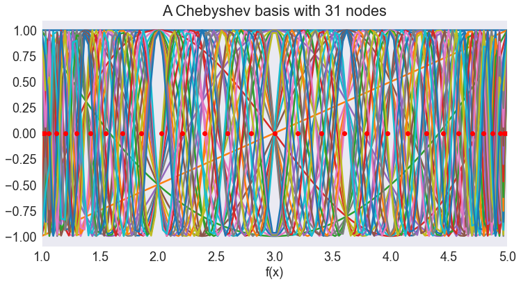
Approximation structure
n, a, b = 31, 1, 5
F = BasisChebyshev(n, a, b, y=5*np.ones(n), labels=['f(x)'])  # define basis functions
x = F.nodes                  # compute standard nodes
F.plot()

Residual function
def resid(c):
    F.c = c  # update basis coefficients
    y = F(x) # interpolate at basis nodes x
    return y ** -2 + y ** -5 - 2 * x
Compute function inverse
c0 = np.zeros(n)  # set initial guess for coeffs
c0[0] = 0.2
problem = NLP(resid)
F.c = problem.broyden(c0)  # compute coeff by Broyden's method
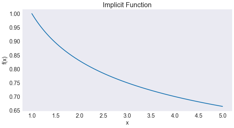
Plot function inverse
n = 1000
x = np.linspace(a, b, n)
r = resid(F.c)

fig1, ax = plt.subplots()
ax.set(title='Implicit Function',
       xlabel='x',
       ylabel='f(x)')
ax.plot(x, F(x));
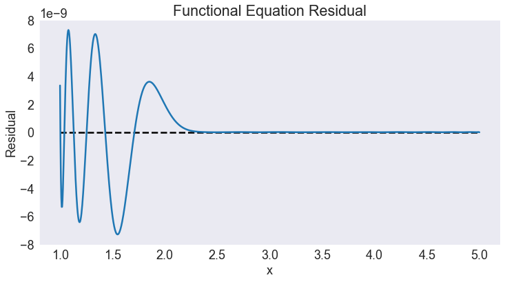
Plot residual
fig2, ax = plt.subplots()
ax.set(title='Functional Equation Residual',
         xlabel='x',
         ylabel='Residual')
ax.hlines(0, a, b, 'k', '--')
ax.plot(x, r);