Hard nonlinear complementarity problem with Billup’s function
Contents
Hard nonlinear complementarity problem with Billup’s function
Randall Romero Aguilar, PhD
This demo is based on the original Matlab demo accompanying the Computational Economics and Finance 2001 textbook by Mario Miranda and Paul Fackler.
Original (Matlab) CompEcon file: demslv09.m
Running this file requires the Python version of CompEcon. This can be installed with pip by running
!pip install compecon --upgrade
Last updated: 2022-Sept-05
About
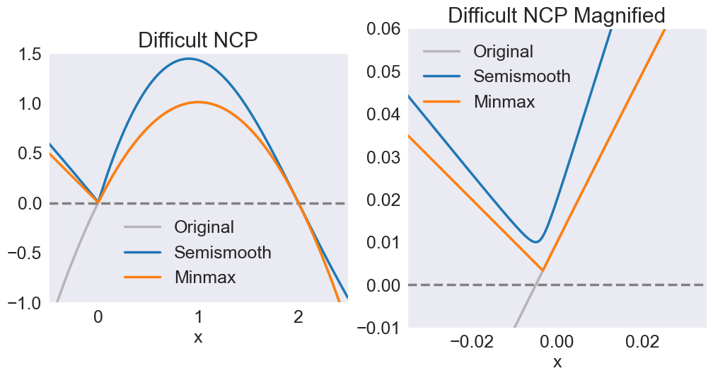
Solve hard nonlinear complementarity problem on R using semismooth and minmax methods. Problem involves Billup’s function. Minmax formulation fails semismooth formulation suceeds.
The function to be solved is $\(f(x) = 1.01 - (1- x)^2\)\( where \)x \geq 0\(. Notice that \)f(x)\( has roots \)1\pm\sqrt{1.01}$
Preliminary tasks
import numpy as np
import pandas as pd
import matplotlib.pyplot as plt
from numpy.linalg import norm
from compecon import MCP, tic, toc, nodeunif
Billup’s function roots are
roots = 1 + np.sqrt(1.01), 1 - np.sqrt(1.01)
print(roots)
(2.004987562112089, -0.00498756211208895)
Set up the problem
The class MCP is used to represent mixed-complementarity problems. To create one instance, we define the objective function and the boundaries \(a\) and \(b\) such that for \(a \leq x \leq b\)
def billups(x):
    fval = 1.01 - (1 - x) ** 2
    return fval, 2*(1 - x )

a = 0
b = np.inf

Billups = MCP(billups, a, b)
Solve by applying Newton method
Using minmax formulation Initial guess is \(x=0\)
t1 = tic()
x1 = Billups.newton(0.0, transform='minmax')
t1 = 100*toc(t1)
n1 = norm(Billups.minmax(x1))
Using semismooth formulation
t2 = tic()
x2 = Billups.newton(0.0, transform='ssmooth')
t2 = 100*toc(t2)
n2 = norm(Billups.minmax(x2))
Print results
Hundreds of seconds required to solve hard nonlinear complementarity problem using Newton minmax and semismooth formulations
results = pd.DataFrame.from_records(
    [('Newton minmax',t1, n1, x1),
     ('Newton semismooth', t2, n2, x2)],
    columns = ['Algorithm', 'Time', 'Norm', 'x']
    ).set_index('Algorithm')

results.style.format(precision=3, subset=['Time', 'x'])
| Time | Norm | x | |
|---|---|---|---|
| Algorithm | |||
| Newton minmax | 15.495 | 0.010000 | 0.000 |
| Newton semismooth | 9.697 | 0.010000 | 0.000 |
Plot results
Here we use the methods ssmooth and minmax from class MCP to compute the semi-smooth and minimax transformations.
original = {'label':'Original', 'alpha':0.5, 'color':'gray'}
xls = [[-0.5, 2.5], [-0.035, 0.035]]
yls = [[-1, 1.5], [-0.01, 0.06]]
ttls = 'Difficult NCP', 'Difficult NCP Magnified'

fig, axs = plt.subplots(1, 2, figsize=[12,6])
for xl, yl, ttl, ax in zip(xls, yls, ttls, axs):
    a, b = xl
    x = np.linspace(a, b, 500)
    ax.set(title=ttl,
           xlabel='x',
           ylabel='',
           xlim=xl,
           ylim=yl,
           aspect=1)
    ax.hlines(0, a, b, 'gray', '--')
    ax.plot(x, billups(x)[0], **original)
    ax.plot(x, Billups.ssmooth(x), label='Semismooth')
    ax.plot(x, Billups.minmax(x), label='Minmax')
    ax.legend(loc='best')

