Mine management model
Contents
Mine management model
Randall Romero Aguilar, PhD
This demo is based on the original Matlab demo accompanying the Computational Economics and Finance 2001 textbook by Mario Miranda and Paul Fackler.
Original (Matlab) CompEcon file: demddp03.m
Running this file requires the Python version of CompEcon. This can be installed with pip by running
!pip install compecon --upgrade
Last updated: 2021-Oct-01
About
A mine operator must decide how much ore to extract from a mine that will be shut down and abandoned after \(T\) years of operation. The price of extracted ore is \(p\) dollars per ton, and the total cost of extracting \(x\) tons of ore in any year, given that the mine contains \(s\) tons at the beginning of the year, is \(c(s, x)\) dollars. The mine currently contains \(\bar{s}\) tons of ore. Assuming the amount of ore extracted in any year must be an integer number of tons, what extraction schedule maximizes profits?
Initial tasks
import numpy as np
import pandas as pd
from compecon import DDPmodel, getindex
Model Parameters
Assuming a market price \(p=1\), initial stock of ore \(\bar{s}=100\), and annual discount factor \(\delta = 0.9\)
price = 1
sbar  = 100
delta = 0.9
State Space
This is a finite horizon, deterministic model with time \(t\) measured in years. The state variable \(s \in \{0, 1, 2, \dots, \bar{s}\}\) is the amount of ore remaining in the mine at the beginning of the year, measured in tons.
S = np.arange(sbar + 1)      # vector of states
n = S.size                   # number of states
Action Space
The action variable \(x \in \{0, 1, 2, \dots, s\}\) is the amount of ore extracted over the year, measured in tons.
X = np.arange(sbar + 1)      # vector of actions
m = X.size                   # number of actions
Reward Function
The reward function is \(f(s, x) = px − c(s, x)\). The cost of extraction is \(c(s, x) = \frac{x^2}{1+s}\).
Here, the reward is set to negative infinity if the extraction level exceeds the available stock in order to preclude the choice of an infeasible action:
f = np.full((m, n), -np.inf)
for c, s in enumerate(S):
    for r, x in enumerate(X):
        if x <= s:
            f[r, c] = price * x - (x ** 2) / (1 + s)
State Transition Function
The state transition function is \(g(s, x) = s − x\)
Here, the routine getindex is used to find the index of the following period’s state.
g = np.empty_like(f)
for r, x in enumerate(X):
    snext = S - x
    g[r] = getindex(snext, S)
Model Structure
The value of the mine, given that it contains \(s\) tons of ore at the beginning of year \(t\), satisfies the Bellman equation
subject to the terminal condition \(V_{T+1}(s) = 0\)
To solve and simulate this model, use the CompEcon class DDPmodel.
model = DDPmodel(f, g, delta)
model.solve()
A deterministic discrete state, discrete action, dynamic model.
There are 101 possible actions over 101 possible states
By default, the solve() method uses Newton’s algorithm. This and other default settings can be changed when solving the model. For example,
model.solve(algorithm='funcit', print=True)
solves the model by function iteration, printing a summary of each iteration to screen.
In either case, solve() updates the model itself, storing the \(n\) vector of values .value, the \(n\) vector of optimal actions .policy, and the \(n\times n\) controlled state .transition probability.
solution = pd.DataFrame({
    'Stock': S,
    'Extraction': X[model.policy],
    'Value': model.value}).set_index('Stock')
Analysis
Simulate Model
The path followed by the stock level over time is computed by the simulate() method. Here, the simulation assumes an initial stock level of 100 and 15 years in duration.
sinit = S.max()
nyrs = 15
t = np.arange(nyrs + 1)
spath, xpath = model.simulate(sinit, nyrs)

simul = pd.DataFrame({
    'Year': t,
    'Stock': S[spath],
    'Extraction': X[xpath]}).set_index('Year')
simul
| Stock | Extraction | |
|---|---|---|
| Year | ||
| 0 | 100 | 24 |
| 1 | 76 | 18 |
| 2 | 58 | 14 |
| 3 | 44 | 11 |
| 4 | 33 | 8 |
| 5 | 25 | 6 |
| 6 | 19 | 5 |
| 7 | 14 | 3 |
| 8 | 11 | 3 |
| 9 | 8 | 2 |
| 10 | 6 | 2 |
| 11 | 4 | 1 |
| 12 | 3 | 1 |
| 13 | 2 | 1 |
| 14 | 1 | 1 |
| 15 | 0 | 0 |
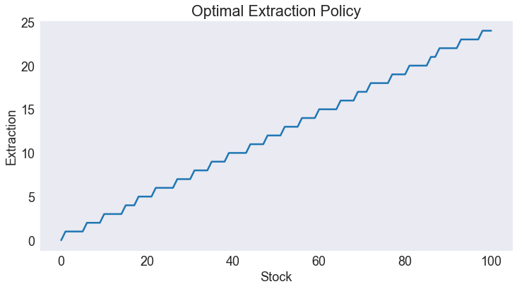
Plot Optimal Policy
ax = solution['Extraction'].plot(title='Optimal Extraction Policy')
ax.set(ylabel='Extraction');

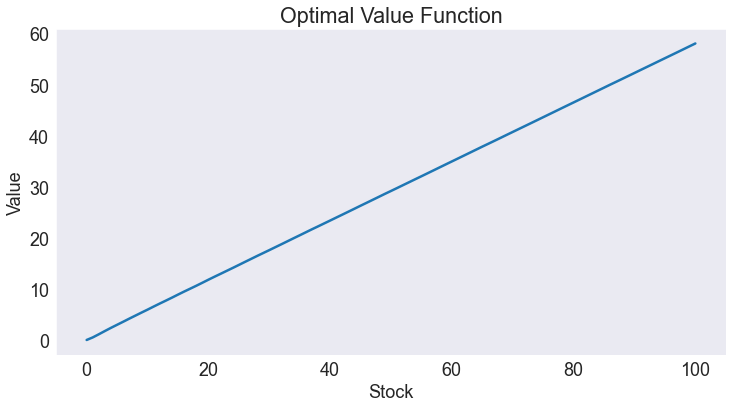
Plot Value Function
The value of the firm is very nearly proportional to the stock level.
ax = solution['Value'].plot(title='Optimal Value Function')
ax.set(ylabel='Value');

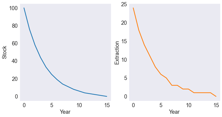
Plot State and Extraction Path
As seen in this figure, the content of the mine is optimally exhausted in 15 years.
ax = simul.plot(subplots=True, layout=[1,2], legend=None)
for i, lab in enumerate(simul.columns):
    ax[0, i].set(ylabel=lab);

