Monopolist’s Effective Supply Function
Contents
Monopolist’s Effective Supply Function
Randall Romero Aguilar, PhD
This demo is based on the original Matlab demo accompanying the Computational Economics and Finance 2001 textbook by Mario Miranda and Paul Fackler.
Original (Matlab) CompEcon file: demapp10.m
Running this file requires the Python version of CompEcon. This can be installed with pip by running
!pip install compecon --upgrade
Last updated: 2022-Oct-22
Initial tasks
import numpy as np
import matplotlib.pyplot as plt
from compecon import BasisChebyshev, NLP
Residual Function
def resid(c):
    Q.c = c
    q = Q(p)
    marginal_income = p + q / (-3.5 * p **(-4.5))
    marginal_cost = np.sqrt(q) + q ** 2
    return  marginal_income - marginal_cost
Approximation structure
n, a, b = 21, 0.5, 2.5
Q = BasisChebyshev(n, a, b)
c0 = np.zeros(n)
c0[0] = 2
p = Q.nodes
Solve for effective supply function
monopoly = NLP(resid)
Q.c = monopoly.broyden(c0)
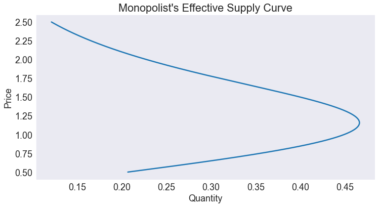
Plot effective supply
nplot = 1000
p = np.linspace(a, b, nplot)
rplot = resid(Q.c)
fig1, ax = plt.subplots()
ax.set(title="Monopolist's Effective Supply Curve",
       xlabel='Quantity',
       ylabel='Price')
ax.plot(Q(p), p);
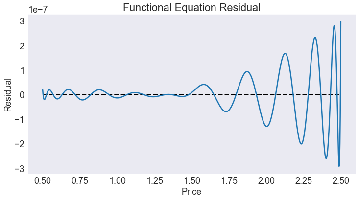
Plot residual
fig2, ax = plt.subplots()
ax.set(title='Functional Equation Residual',
       xlabel='Price',
       ylabel='Residual')
ax.hlines(0, a, b, 'k', '--')
ax.plot(p, rplot);