Illustrates linear complementarity problem
Contents
Illustrates linear complementarity problem
Randall Romero Aguilar, PhD
This demo is based on the original Matlab demo accompanying the Computational Economics and Finance 2001 textbook by Mario Miranda and Paul Fackler.
Original (Matlab) CompEcon file: demslv10.m
Running this file requires the Python version of CompEcon. This can be installed with pip by running
!pip install compecon --upgrade
Last updated: 2021-Oct-01
import matplotlib.pyplot as plt
plt.style.use('seaborn')
def basicsubplot(ax, title, yvals,solution):
    ax.set(title=title,
           xlabel='',
           ylabel='',
           xlim=[-0.05,1.05],
           ylim=[-2,2],
           xticks=[0,1],
           xticklabels=['a','b'],
           yticks=[-2,0,2],
           yticklabels=['','0',''])

    ax.plot([0,1],[0,0],'k-',linewidth=1.5)
    ax.plot([0,0],[-2,2],'k:',linewidth=2.5)
    ax.plot([1,1],[-2,2],'k:',linewidth=2.5)
    ax.plot([0, 1],yvals)
    ax.plot(solution[0], solution[1],'r.', ms=18)
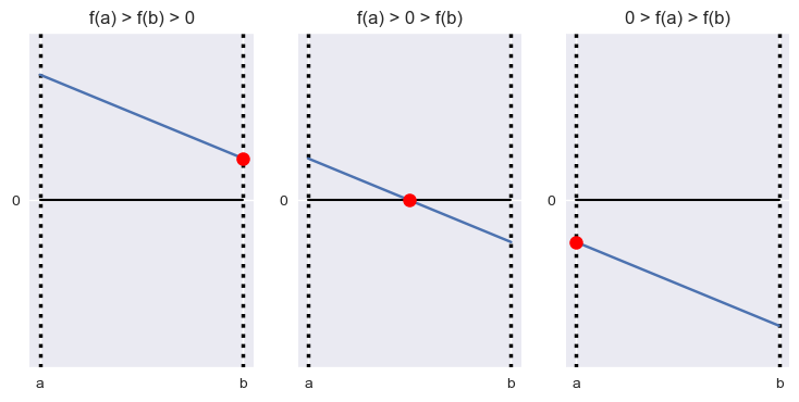
Possible Solutions to Complementarity Problem, \(f\) Strictly Decreasing
fig1, axs = plt.subplots(1,3,figsize=[9,4])
basicsubplot(axs[0],'f(a) > f(b) > 0', [1.5, 0.5], [1.0,0.5])
basicsubplot(axs[1],'f(a) > 0 > f(b)', [0.5, -0.5], [0.5,0.0])
basicsubplot(axs[2],'0 > f(a) > f(b)', [-0.5, -1.5],[0.0,-0.5])
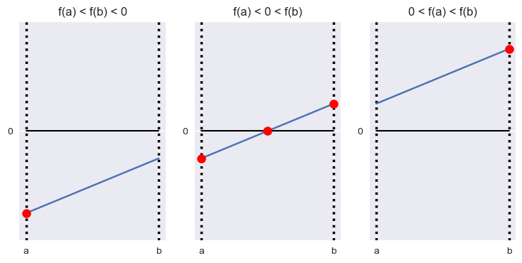
Possible Solutions to Complementarity Problem, \(f\) Strictly Increasing
fig2, axs = plt.subplots(1,3,figsize=[9,4])
basicsubplot(axs[0],'f(a) < f(b) < 0', [-1.5, -0.5], [0.0,-1.5])
basicsubplot(axs[1],'f(a) < 0 < f(b)', [-0.5, 0.5], [0.5,0.0])
basicsubplot(axs[2],'0 < f(a) < f(b)', [0.5, 1.5],[1.0,1.5])
axs[1].plot(0.0,-0.5,'r.',ms=18)
axs[1].plot(1.0,0.5,'r.',ms=18)
[<matplotlib.lines.Line2D at 0x18b70cc9b80>]