Public Renewable Resource Model
Contents
Public Renewable Resource Model
Randall Romero Aguilar, PhD
This demo is based on the original Matlab demo accompanying the Computational Economics and Finance 2001 textbook by Mario Miranda and Paul Fackler.
Original (Matlab) CompEcon file: demdp01.m
Running this file requires the Python version of CompEcon. This can be installed with pip by running
!pip install compecon --upgrade
Last updated: 2022-Oct-23
About
Welfare maximizing social planner must decide how much of a renewable resource to harvest.
States
s quantity of stock available
Actions
q quantity of stock harvested
Parameters
\(\alpha\) growth function parameter
\(\beta\) growth function parameter
\(\gamma\) relative risk aversion
\(\kappa\) unit cost of harvest
\(\delta\) discount factor
import numpy as np
import matplotlib.pyplot as plt
from compecon import BasisChebyshev, DPmodel, DPoptions, qnwnorm
Model parameters
α, β, γ, κ, δ = 4.0, 1.0, 0.5, 0.2, 0.9
Steady-state
The steady-state values for this model are
sstar = (α**2 - 1/δ**2)/(2*β)     # steady-state stock
qstar = sstar - (δ*α-1)/(δ*β) # steady-state action

print('Steady-State')
print(f"\t{'Stock':12s} = {sstar:8.4f}")
print(f"\t{'Harvest':12s} = {qstar:8.4f}")
Steady-State
	Stock        =   7.3827
	Harvest      =   4.4938
Numeric results
State space
The state variable is s=”Stock”, which we restrict to \(s\in[6, 9]\).
Here, we represent it with a Chebyshev basis, with \(n=8\) nodes.
n, smin, smax = 8, 6, 9
basis = BasisChebyshev(n, smin, smax, labels=['Stock'])
Action space
The choice variable q=”Harvest” must be nonnegative.
def bounds(s, i=None, j=None):
    return np.zeros_like(s), s[:]
Reward function
The reward function is the utility of harvesting \(q\) units.
def reward(s, q, i=None, j=None):
    u = (q**(1-γ))/(1-γ)-κ*q
    ux= q**(-γ)-κ
    uxx = -γ*q**(-γ-1)

    return u, ux, uxx
State transition function
Next period, the stock will be equal that is \(s' = \alpha (s-q) - 0.5\beta(s-q)^2\)
def transition(s, q, i=None, j=None, in_=None, e=None):
    sq = s-q
    g = α*sq - 0.5*β*sq**2
    gx = -α + β*sq
    gxx = -β*np.ones_like(s)
    return g, gx, gxx
Model structure
The value of wealth \(s\) satisfies the Bellman equation
To solve and simulate this model,use the CompEcon class DPmodel
model = DPmodel(basis, reward, transition, bounds,
                       x=['Harvest'],
                       discount=δ)
Solving the model
Solving the growth model by collocation
S = model.solve()
Solving infinite-horizon model collocation equation by Newton's method
iter change       time
------------------------------
   0       1.4e+01    0.0000
   1       1.9e+01    0.0157
   2       3.7e-01    0.0157
   3       1.1e-03    0.0157
   4       1.5e-08    0.0312
   5       1.7e-14    0.0312
Elapsed Time =    0.03 Seconds
DPmodel.solve returns a pandas DataFrame with the following data:
S.head()
| Stock | value | resid | Harvest | |
|---|---|---|---|---|
| Stock | ||||
| 6.000000 | 6.000000 | 32.985613 | 6.795958e-09 | 3.349254 |
| 6.037975 | 6.037975 | 32.998722 | -1.561702e-09 | 3.379828 |
| 6.075949 | 6.075949 | 33.011736 | -5.604697e-09 | 3.410456 |
| 6.113924 | 6.113924 | 33.024658 | -6.686079e-09 | 3.441138 |
| 6.151899 | 6.151899 | 33.037489 | -5.868451e-09 | 3.471872 |
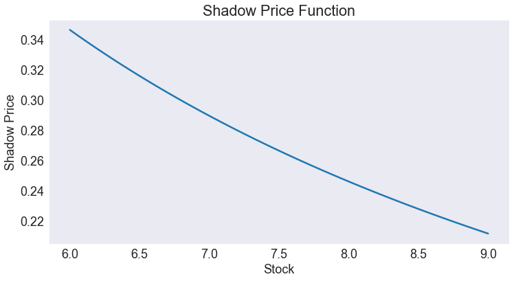
We are also interested in the shadow price of wealth (the first derivative of the value function).
S['shadow price'] = model.Value(S['Stock'],1)
Plotting the results
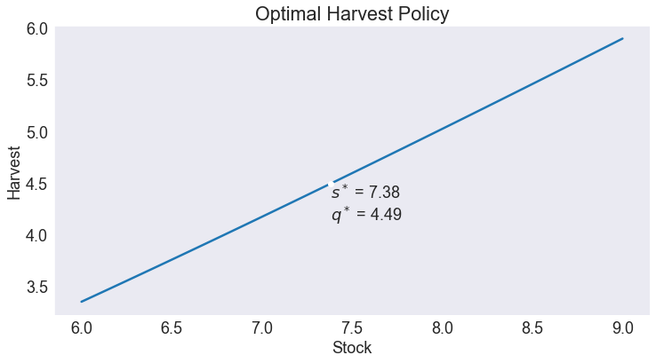
Optimal Policy
fig1, ax = plt.subplots()
ax.set(title='Optimal Harvest Policy', xlabel='Stock', ylabel='Harvest')
ax.plot(S['Harvest'])

ax.plot(sstar, qstar,'wo')
ax.annotate(f"$s^*$ = {sstar:.2f}\n$q^*$ = {qstar:.2f}",[sstar, qstar], va='top');
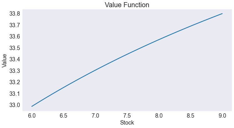
Value Function
fig2, ax = plt.subplots()

ax.set(title='Value Function', xlabel='Stock', ylabel='Value')
ax.plot(S.value);
Shadow Price Function
fig3, ax = plt.subplots()
ax.set(title='Shadow Price Function', xlabel='Stock', ylabel='Shadow Price')
ax.plot(S['shadow price']);
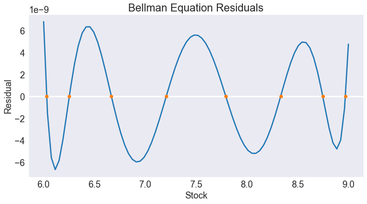
Residual
fig4, ax = plt.subplots()
ax.set(title='Bellman Equation Residuals', xlabel='Stock', ylabel='Residual')
ax.axhline(0,color='w')
ax.plot(S['resid'])
ax.plot(basis.nodes[0], np.zeros_like(basis.nodes[0]), lw=0, marker='.', ms=12)
ax.ticklabel_format(style='sci', axis='y', scilimits=(-1,1))
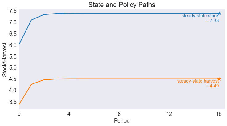
Simulating the model
We simulate 16 periods of the model starting from \(s=s_{\min}\)
T = 16
data = model.simulate(T, smin)
Simulated State and Policy Paths
opts = dict(ha='right', va='top', fontsize='small')

fig5, ax = plt.subplots()

ax.set(title='State and Policy Paths',
       xlabel='Period',
       ylabel='Stock/Harvest',
       xlim=[0, T + 0.5],
       xticks=range(0,T+1,4))

ax.plot(data[['Stock', 'Harvest']])

ax.plot(T, sstar, color='C0', marker='*', ms=12)
ax.annotate(f"steady-state stock\n = {sstar:.2f}", [T, sstar-0.01], color='C0', **opts)

ax.plot(T, qstar, color='C1', marker='*', ms=12)
ax.annotate(f"steady-state harvest\n = {qstar:.2f}", [T, qstar-0.01], color='C1', **opts);