Major Distribution CDFs and PDFs
Contents
Major Distribution CDFs and PDFs
Randall Romero Aguilar, PhD
This demo is based on the original Matlab demo accompanying the Computational Economics and Finance 2001 textbook by Mario Miranda and Paul Fackler.
Original (Matlab) CompEcon file: demmath03.m
Running this file requires the Python version of CompEcon. This can be installed with pip by running
!pip install compecon --upgrade
Last updated: 2022-Oct-23
import numpy as np
import matplotlib.pyplot as plt
plt.style.use('seaborn')
Change some settings for the plots
font = {'family' : 'normal',
        'weight' : 'bold',
        'size'   : 24}

from matplotlib import rc
rc('font', **font)
rc('text', usetex=True)
First define a layout function to help format the plots
CONTINUOUS DISTRIBUTIONS
from scipy.stats import norm, lognorm, beta, gamma, expon, chi2, f, t, logistic
n = 400
def plot_distribution(x, ypdf, ycdf, p=None, q=None):
    xr = [min(x), max(x)]
    fig, (ax0, ax1) = plt.subplots(1,2, figsize=[12,5])
    ax0.set(title='Probability Density', xlabel='x', ylabel='', xlim=xr)
    ax0.plot(x, ypdf)

    ax1.set(title='Cumulative Probability', xlabel='x', ylabel='', xlim=xr)
    ax1.plot(x, ycdf)

    if p is not None:
        ax1.plot([xr[0], q, q], [p, p, 0.0], color='C1', linestyle='dotted')
        ax1.plot(q, 0, 'k', marker='.', markersize=8)
        ax1.annotate('  $x_{%.2f} = %.2f$' % (p, q), [q, 0.0], va='center', fontsize=14, color='C1')
        ax1.plot(xr[0], p, 'k', marker='.', markersize=8)
        ax1.annotate(f'{p:.2f}  ', [xr[0], p], va='center', ha='right', fontsize=14, color='C1')
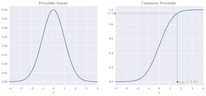
Standard Normal distribution
x =  np.linspace(-4, 4, n)
p = 0.95
plot_distribution(x, norm.pdf(x), norm.cdf(x), p, norm.ppf(p))

print(f'Prob[-1 < x <= 1] = {norm.cdf(1) - norm.cdf(-1):.4f}')
print(f'Prob[-2 < x <= 2] = {norm.cdf(2) - norm.cdf(-2):.4f}')

print(f'\nProb[{norm.ppf(0.05):.3f} < X <= {norm.ppf(0.95):.3f}] = 0.90')
print(f'Prob[{norm.ppf(0.025):.3f} < X <= {norm.ppf(0.975):.3f}] = 0.95')
print(f'Prob[{norm.ppf(0.005):.3f} < X <= {norm.ppf(0.995):.3f}] = 0.99')
Prob[-1 < x <= 1] = 0.6827
Prob[-2 < x <= 2] = 0.9545

Prob[-1.645 < X <= 1.645] = 0.90
Prob[-1.960 < X <= 1.960] = 0.95
Prob[-2.576 < X <= 2.576] = 0.99
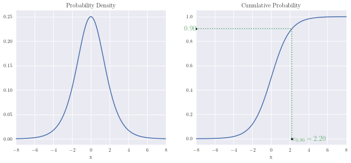
Logistic distribution
x =  np.linspace(-8, 8, n)
p = 0.9
plot_distribution(x, logistic.pdf(x) , logistic.cdf(x), p, logistic.ppf(p))

print(f'Prob[-1 < x <= 1] = {logistic.cdf(1) - logistic.cdf(-1):.4f}')
print(f'Prob[-2 < x <= 2] = {logistic.cdf(2) - logistic.cdf(-2):.4f}')

print(f'\nProb[{logistic.ppf(0.05):.3f} < X <= {logistic.ppf(0.95):.3f}] = 0.90')
print(f'Prob[{logistic.ppf(0.025):.3f} < X <= {logistic.ppf(0.975):.3f}] = 0.95')
print(f'Prob[{logistic.ppf(0.005):.3f} < X <= {logistic.ppf(0.995):.3f}] = 0.99')
Prob[-1 < x <= 1] = 0.4621
Prob[-2 < x <= 2] = 0.7616

Prob[-2.944 < X <= 2.944] = 0.90
Prob[-3.664 < X <= 3.664] = 0.95
Prob[-5.293 < X <= 5.293] = 0.99
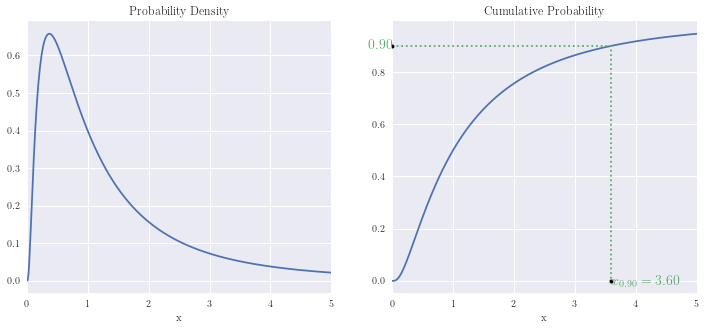
Lognormal distribution
mu, var = 0, 1
params = {'s': np.sqrt(var),
          'scale': np.exp(mu)}

x =  np.linspace(0, 5, n)
p = 0.9
plot_distribution(x, lognorm.pdf(x, **params), lognorm.cdf(x, **params), p, lognorm.ppf(p, **params))

print(f'\nProb[0 < X <= {lognorm.ppf(0.90, **params):.3f}] = 0.90')
print(f'Prob[0 < X <= {lognorm.ppf(0.95, **params):.3f}] = 0.95')
print(f'Prob[0 < X <= {lognorm.ppf(0.99, **params):.3f}] = 0.99')
Prob[0 < X <= 3.602] = 0.90
Prob[0 < X <= 5.180] = 0.95
Prob[0 < X <= 10.240] = 0.99
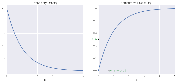
Exponential distribution
x =  np.linspace(0, 5, n)
p = 0.5
plot_distribution(x, expon.pdf(x), expon.cdf(x), p, expon.ppf(p))


print(f'\nProb[0 < X <= {expon.ppf(0.90):.3f}] = 0.90')
print(f'Prob[0 < X <= {expon.ppf(0.95):.3f}] = 0.95')
print(f'Prob[0 < X <= {expon.ppf(0.99):.3f}] = 0.99')
Prob[0 < X <= 2.303] = 0.90
Prob[0 < X <= 2.996] = 0.95
Prob[0 < X <= 4.605] = 0.99
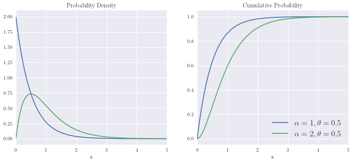
Gamma Distribution
x =  np.linspace(0, 5, n)
plot_distribution(x, np.array([gamma.pdf(x, 1,scale=0.5), gamma.pdf(x,2, scale=0.5)]).T,
                  np.array([gamma.cdf(x, 1, scale=0.5), gamma.cdf(x,2, scale=0.5)]).T)
plt.legend([r'$\alpha=1, \theta=0.5$',
           r'$\alpha=2, \theta=0.5$'], fontsize=16)
<matplotlib.legend.Legend at 0x1e4ce931fa0>
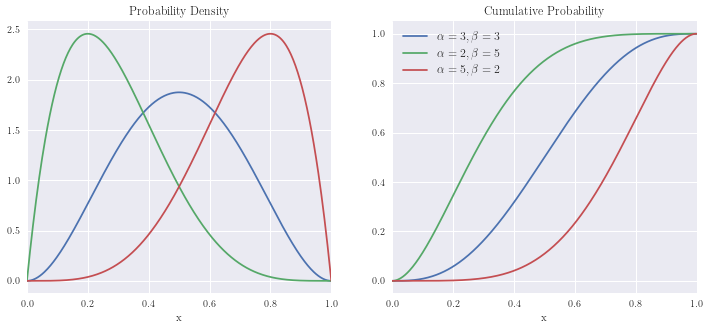
Beta Distribution
x =  np.linspace(0, 1, n)
plot_distribution(x, np.array([beta.pdf(x, 3,3), beta.pdf(x,2,5), beta.pdf(x,5,2)]).T,
                  np.array([beta.cdf(x, 3,3), beta.cdf(x,2,5), beta.cdf(x,5,2)]).T)
plt.legend([r'$\alpha=3, \beta=3$', r'$\alpha=2, \beta=5$', r'$\alpha=5, \beta=2$'], fontsize=12)
<matplotlib.legend.Legend at 0x1e4ce901fa0>
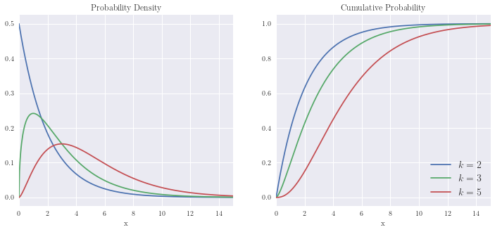
Chi-squared distribution
x =  np.linspace(0, 15, n)
plot_distribution(x, np.array([chi2.pdf(x, 2), chi2.pdf(x,3), chi2.pdf(x,5)]).T,
                  np.array([chi2.cdf(x, 2), chi2.cdf(x,3), chi2.cdf(x,5)]).T)
plt.legend([r'$k=2$', r'$k=3$', r'$k=5$'], fontsize=14)
<matplotlib.legend.Legend at 0x1e4cea34130>
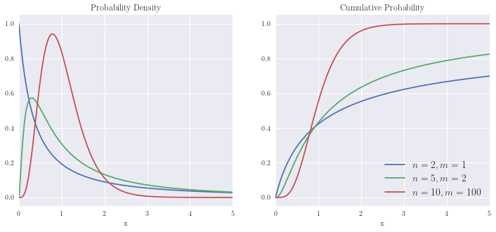
F distribution
x =  np.linspace(0, 5, n)
plot_distribution(x, np.array([f.pdf(x, 2,1), f.pdf(x,5,2), f.pdf(x,10,100)]).T,
                  np.array([f.cdf(x, 2,1), f.cdf(x,5,2), f.cdf(x,10, 100)]).T)
plt.legend([r'$n=2, m=1$', r'$n=5, m=2$', r'$n=10, m=100$'], fontsize=14)
<matplotlib.legend.Legend at 0x1e4cd63a8b0>
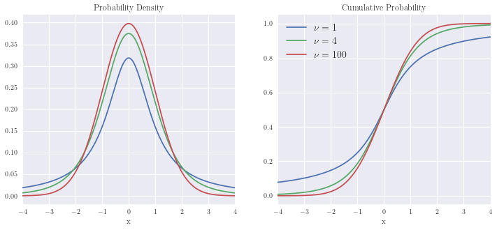
Student’s- t distribution
x =  np.linspace(-4, 4, n)
plot_distribution(x, np.array([t.pdf(x, 1), t.pdf(x,4), t.pdf(x,100)]).T,
                  np.array([t.cdf(x, 1), t.cdf(x,4), t.cdf(x, 100)]).T)
plt.legend([r'$\nu=1$', r'$\nu=4$', r'$\nu=100$'], fontsize=14)
<matplotlib.legend.Legend at 0x1e4ccf7ce20>
DISCRETE DISTRIBUTIONS
from scipy.stats import binom, geom, poisson
def plot_ddistribution(x, ypdf, x2, ycdf):
    fig, (ax0, ax1) = plt.subplots(1,2, figsize=[12,5])
    ax0.set(title='Probability Density', xlabel='x', ylabel='', xticks=x)
    ax0.bar(x, ypdf)

    ax1.set(title='Cumulative Probability', xlabel='x', ylabel='', xticks=x)
    ax1.step(x2, ycdf)
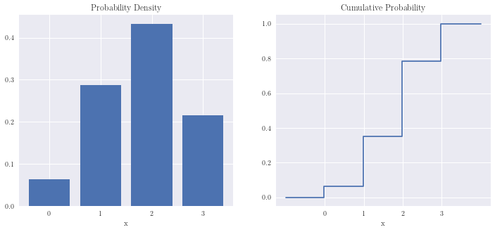
Binomial distribution
n, p = 3, 0.6
x =  np.arange(n+1)
x2 = np.linspace(-1, n+1, 60*(n+2)+1)
plot_ddistribution(x, binom.pmf(x, n, p), x2, binom.cdf(x2, n,p))
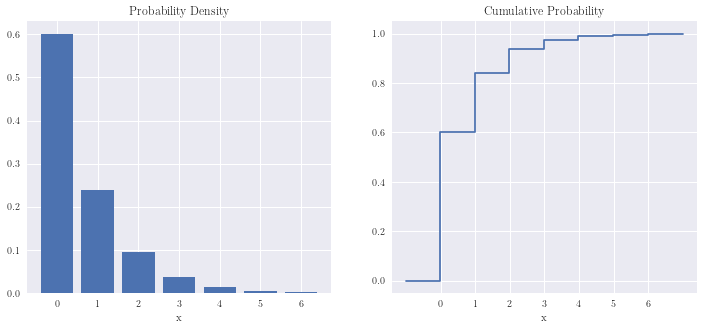
Geometric distribution
n, p = 6, 0.6
x =  np.arange(n+1)
x2 = np.linspace(-1, n+1, 60*(n+2)+1)
plot_ddistribution(x, geom.pmf(x, p, loc=-1), x2, geom.cdf(x2, p, loc=-1))
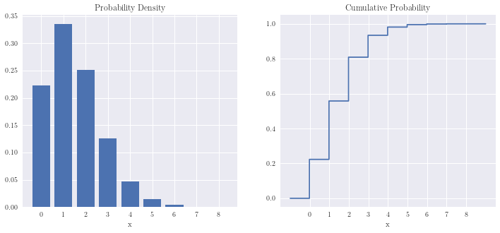
Poisson distribution
n, lambda_ = 8, 1.5
x =  np.arange(n+1)
x2 = np.linspace(-1, n+1, 60*(n+2)+1)
plot_ddistribution(x, poisson.pmf(x, lambda_), x2, poisson.cdf(x2, lambda_))