Convergence rates for different NLP methods
Contents
Convergence rates for different NLP methods
Randall Romero Aguilar, PhD
This demo is based on the original Matlab demo accompanying the Computational Economics and Finance 2001 textbook by Mario Miranda and Paul Fackler.
Original (Matlab) CompEcon file: demslv12.m
Running this file requires the Python version of CompEcon. This can be installed with pip by running
!pip install compecon --upgrade
Last updated: 2022-Sept-05
About
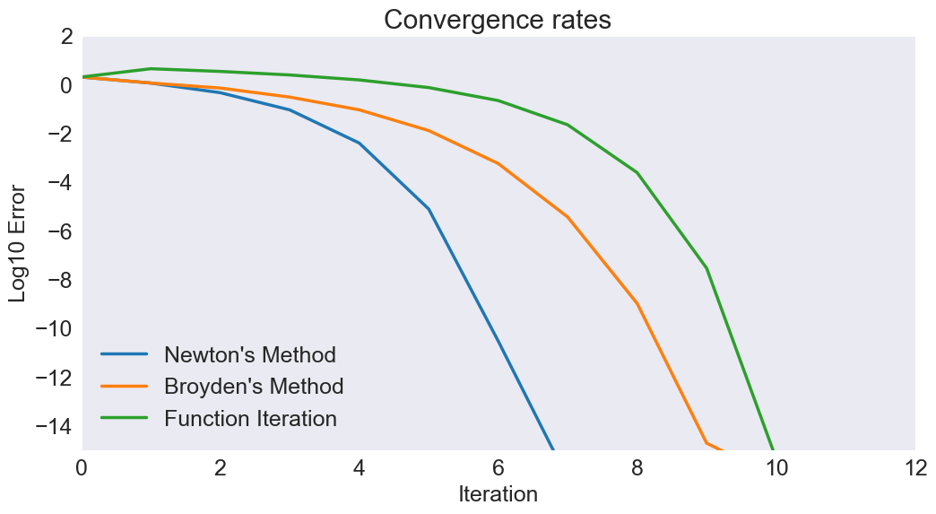
This demo shows how quickly different NLP methods converge to a solution. In particular, we look for the root of $\(f(x) = \exp(x) - 1\)$
starting with a guess \(x_0 = 2\). The true solution is \(x = 0\).
import numpy as np
import matplotlib.pyplot as plt
from compecon import NLP
Define a NLP problem
Here, we set convergence tolerance tol=1e-20 and the option all_x=True to record all values taken by \(x\) from the initial guess x0=2.0 to the final solution. These values will be stored in the .x_sequence attribute.
We also define err to compute the base-10 logarithm of the error (the gap between the current iteration and the solution).
A = NLP(lambda x: (np.exp(x)-1, np.exp(x)), all_x=True, tol=1e-20)
err = lambda z: np.log10(np.abs(z)).flatten()
x0 = 2.0
Solve the problem
* Using Newton’s method
A.newton(x0)
err_newton = err(A.x_sequence.values)
* Using Broyden’s method
A.broyden(x0)
err_broyden = err(A.x_sequence.values)
* Using function iteration
This method finds a zero of \(f(x)\) by looking for a fixpoint of \(g(x) = x-f(x)\).
A.funcit(x0)
err_funcit = err(A.x_sequence.values)
Plot results
fig, ax = plt.subplots()
ax.set(title='Convergence rates',
       xlabel='Iteration',
       ylabel='Log10 Error',
       xlim=[0, 12],
       ylim=[-15, 2])
ax.plot(err_newton, label="Newton's Method")
ax.plot(err_broyden, label="Broyden's Method")
ax.plot(err_funcit, label="Function Iteration")
ax.legend(loc='lower left');