Area under 1-D and 2-D curves, various methods
Contents
Area under 1-D and 2-D curves, various methods
Randall Romero Aguilar, PhD
This demo is based on the original Matlab demo accompanying the Computational Economics and Finance 2001 textbook by Mario Miranda and Paul Fackler.
Original (Matlab) CompEcon file: demqua03.m
Running this file requires the Python version of CompEcon. This can be installed with pip by running
!pip install compecon --upgrade
Last updated: 2022-Oct-23
About
Uni- and bi-vaiariate integration using Newton-Cotes, Gaussian, Monte Carlo, and quasi-Monte Carlo quadrature methods.
Initial tasks
import numpy as np
from compecon import qnwtrap, qnwsimp, qnwlege
import matplotlib.pyplot as plt
import pandas as pd
quadmethods = [qnwtrap, qnwsimp, qnwlege]
Make support function
a, b = -1, 1
nlist = [5, 11, 21, 31]
N = len(nlist)

def quad(func, qnw, n):
    xi, wi = qnw(n,a,b)
    return np.dot(func(xi),wi)
Evaluating
\(\int_{-1}^1e^{-x}dx\)
def f(x):
    return np.exp(-x)

f_quad = np.array([[quad(f, qnw, ni) for qnw in quadmethods] for ni in nlist])
f_true = np.exp(1) - 1/np.exp(1)
f_error = np.log10(np.abs(f_quad/f_true - 1))
Evaluating
\(\int_{-1}^1\sqrt{|x|}dx\)
def g(x):
    return np.sqrt(np.abs(x))

g_quad = np.array([[quad(g, qnw, ni) for qnw in quadmethods] for ni in nlist])
g_true = 4/3
g_error = np.log10(np.abs(g_quad/g_true - 1))
Make table with results
methods = ['Trapezoid rule', "Simpson's rule", 'Gauss-Legendre']
functions = [r'$\int_{-1}^1e^{-x}dx$', r'$\int_{-1}^1\sqrt{|x|}dx$']

results = pd.concat(
    [pd.DataFrame(errors, columns=methods, index=nlist) for errors in (f_error, g_error)],
    keys=functions)

results
| Trapezoid rule | Simpson's rule | Gauss-Legendre | ||
|---|---|---|---|---|
| $\int_{-1}^1e^{-x}dx$ | 5 | -1.683044 | -3.472173 | -9.454795 |
| 11 | -2.477411 | -5.053217 | -14.273349 | |
| 21 | -3.079254 | -6.255789 | -14.675836 | |
| 31 | -3.431396 | -6.959867 | -15.653560 | |
| $\int_{-1}^1\sqrt{|x|}dx$ | 5 | -1.023788 | -1.367611 | -0.870112 |
| 11 | -1.595301 | -1.347900 | -1.351241 | |
| 21 | -2.034517 | -2.414470 | -1.758970 | |
| 31 | -2.293296 | -2.063539 | -2.007803 |
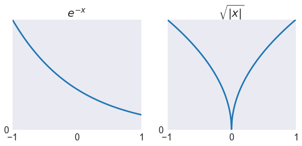
Plot the functions
a, b, n = -1, 1, 301
x = np.linspace(a, b, n)

options = dict(xlim=[a,b], xticks=[-1,0,1], yticks=[0])

fig, axs = plt.subplots(1, 2, figsize=[10,4])
axs[0].plot(x, f(x), linewidth=3)
axs[0].set(title='$e^{-x}$', ylim=[0,f(a)], **options)

axs[1].plot(x, g(x), linewidth=3)
axs[1].set(title='$\sqrt{|x|}$', ylim=[0,g(a)], **options);