Generic IVP Nonlinear ODE Example
Contents
Generic IVP Nonlinear ODE Example
Randall Romero Aguilar, PhD
This demo is based on the original Matlab demo accompanying the Computational Economics and Finance 2001 textbook by Mario Miranda and Paul Fackler.
Original (Matlab) CompEcon file: demode02.m
Running this file requires the Python version of CompEcon. This can be installed with pip by running
!pip install compecon --upgrade
Last updated: 2021-Oct-01
About
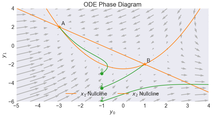
Solve
\[\begin{align*}
\dot{y_0} &= y_0^2 - 2y_1 - a\\
\dot{y_1} &= b - y_0 - y_1
\end{align*}\]
FORMULATION
from compecon import jacobian, ODE

import numpy as np
import pandas as pd
import matplotlib.pyplot as plt
Velocity Function
a =  5
b = -1

def f(x, a, b):
    x1, x2 = x
    return np.array([x1**2 - 2*x2-a, b-x1-x2])
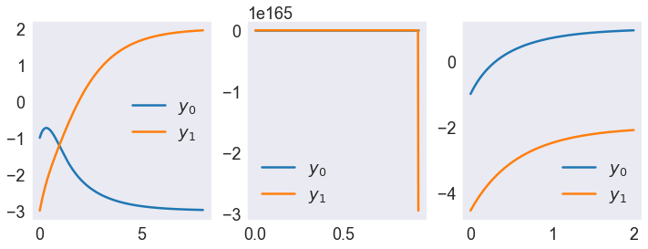
Initial States
xinit = np.array([[-1,-3],[-1,-6], [-1, -4.5578]])
Time Horizons
T = [8, 2, 2]
SOLVE ODE USING RUNGE-KUTTA METHOD (RK4)
Solve for Different Initial Values
N = 1000   # number of time nodes
x = np.zeros([3,N,2])

problems = [ODE(f,t,x0,a,b) for x0, t in zip(xinit, T)]

# Plot Solutions in Time Domain
fig, axs = plt.subplots(1,3, figsize=[12,4])
for problem, ax in zip(problems, axs):
    problem.rk4(N)
    problem.x.plot(ax=ax)
STEADY STATES
# Compute Steady State A
A1 = (-2-np.sqrt(4+4*(2*b+a)))/2
A  = np.array([A1,b-A1])
print('Steady State A = ', A, '-->  Eigenvalues = ', np.linalg.eigvals(jacobian(f,A,a,b)))

# Compute Steady State B
B1 = (-2+np.sqrt(4+4*(2*b+a)))/2
B  = np.array([B1,b-B1])
print('Steady State B = ', B, '-->  Eigenvalues = ', np.linalg.eigvals(jacobian(f,B,a,b)))
Steady State A =  [-3.  2.] -->  Eigenvalues =  [-6.3723 -0.6277]
Steady State B =  [ 1. -2.] -->  Eigenvalues =  [ 2.5616 -1.5616]
PHASE DIAGRAM
# Ploting Limits
x1lim = [-5, 4]
x2lim = [-6, 4]

# Compute Separatrix
T = 10;
problem2 = ODE(f,T,B,a,b)
problem2.spx()

x = np.array([problem.x.values.T for problem in problems])

# Compute Nullclines
x1 = np.linspace(*x1lim, 100)
xnulls = pd.DataFrame({'$x_1$ Nullcline': (x1**2-a)/2,
                       '$x_2$ Nullcline': b-x1},
                     index = x1)

# Plot Phase Diagram
fig, ax =  plt.subplots()

for txt, xy in zip('AB', [A,B]):
    ax.annotate(txt, xy + [0.1,0.2])

for i, xy in enumerate(x[:,:,0]):
    ax.annotate(str(i), xy+[0,0.20], color='C2', ha='center', fontsize=14)

problem.phase(x1lim, x2lim,
              xnulls=xnulls,
              xstst=np.r_[A,B],
              x=x,
              title='ODE Phase Diagram',
              ax=ax,
              animated=5  # requires ffmpeg for video, change to 0 for static image
             )