Deterministic Optimal Economic Growth Model
Contents
Deterministic Optimal Economic Growth Model
Randall Romero Aguilar, PhD
This demo is based on the original Matlab demo accompanying the Computational Economics and Finance 2001 textbook by Mario Miranda and Paul Fackler.
Original (Matlab) CompEcon file: demdoc02.m
Running this file requires the Python version of CompEcon. This can be installed with pip by running
!pip install compecon --upgrade
Last updated: 2021-Oct-01
About
Social benefit maximizing social planner must decide how much society should consume and invest.
State
k capital stock
Control
q consumption rate
Parameters
𝛼 capital share
𝛿 capital depreciation rate
𝜃 relative risk aversion
𝜌 continuous discount rate
Preliminary tasks
Import relevant packages
import pandas as pd
import matplotlib.pyplot as plt
from compecon import BasisChebyshev, OCmodel
Model parameters
𝛼 =  0.4        # capital share
𝛿 =  0.1        # capital depreciation rate
𝜃 =  2.0        # relative risk aversion
𝜌 =  0.05       # continuous discount rate
Approximation structure
n = 21          # number of basis functions
kmin = 1        # minimum state
kmax = 7        # maximum state
basis = BasisChebyshev(n, kmin, kmax, labels=['Capital Stock'])  # basis functions
Steady-state
kstar = ((𝛿+𝜌)/𝛼)**(1/(𝛼-1))       # capital stock
qstar = kstar**𝛼 - 𝛿*kstar         # consumption rate
vstar = ((1/(1-𝜃))*qstar**(1-𝜃))/𝜌 # value
lstar =  qstar ** (-𝜃)             # shadow price

steadystate = pd.Series([kstar, qstar, vstar, lstar],
                       index=['Capital stock', 'Rate of consumption', 'Value Function', 'Shadow Price'])

steadystate
Capital stock           5.127998
Rate of consumption     1.410200
Value Function        -14.182390
Shadow Price            0.502850
dtype: float64
Solve HJB equation by collocation
Initial guess
k = basis.nodes
basis.y = ((𝜌*k)**(1-𝜃))/(1-𝜃)
Define model and solve it.
def control(k, Vk, 𝛼,𝛿,𝜃,𝜌):
    return Vk**(-1/𝜃)

def reward(k, q, 𝛼,𝛿,𝜃,𝜌):
    return (1/(1-𝜃)) * q**(1-𝜃)

def transition(k, q, 𝛼,𝛿,𝜃,𝜌):
    return k**𝛼 - 𝛿*k - q

model = OCmodel(basis, control, reward, transition, rho=𝜌, params=[𝛼,𝛿,𝜃,𝜌])
data = model.solve()
Solving optimal control model
iter change       time
------------------------------
   0       8.4e+00    0.0010
   1       7.8e-01    0.0020
   2       1.5e-01    0.0020
   3       8.1e-03    0.0020
   4       2.9e-05    0.0030
   5       4.4e-10    0.0030
Elapsed Time =    0.00 Seconds
Plots
Optimal policy
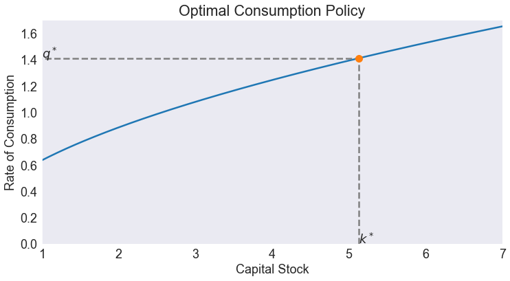
fig, ax = plt.subplots()
data['control'].plot(ax=ax)
ax.set(title='Optimal Consumption Policy',
       xlabel='Capital Stock',
       ylabel='Rate of Consumption',
       xlim=[kmin, kmax])
ax.set_ylim(bottom=0)
ax.hlines(qstar, 0, kstar, colors=['gray'], linestyles=['--'])
ax.vlines(kstar, 0, qstar, colors=['gray'], linestyles=['--'])
ax.annotate('$q^*$', (kmin, qstar))
ax.annotate('$k^*$', (kstar, 0))
ax.plot(kstar, qstar, '.', ms=20);
Value function
fig, ax = plt.subplots()
data['value'].plot(ax=ax)
ax.set(title='Value Function',
       xlabel='Capital Stock',
       ylabel='Lifetime Utility',
       xlim=[kmin, kmax])

lb = ax.get_ylim()[0]
ax.vlines(kstar, lb , vstar, colors=['gray'], linestyles=['--'])
ax.annotate('$k^*$', (kstar, lb))
ax.plot(kstar, vstar, '.', ms=20);

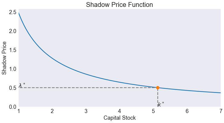
Shadow price
data['shadow'] = model.Value(data.index, 1)

fig, ax = plt.subplots()
data['shadow'].plot(ax=ax)
ax.set(title='Shadow Price Function',
       xlabel='Capital Stock',
       ylabel='Shadow Price',
       xlim=[kmin, kmax])

ax.set_ylim(bottom=0)
ax.hlines(lstar, 0, kstar, colors=['gray'], linestyles=['--'])
ax.vlines(kstar, 0 , lstar, colors=['gray'], linestyles=['--'])
ax.annotate('$\lambda^*$', (kmin, lstar))
ax.annotate('$k^*$', (kstar, 0))
ax.plot(kstar, lstar, '.', ms=20);
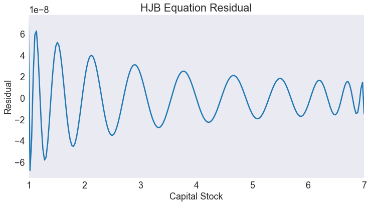
Residual
fig, ax = plt.subplots()
data['resid'].plot(ax=ax)
ax.set(title='HJB Equation Residual',
       xlabel='Capital Stock',
       ylabel='Residual',
       xlim=[kmin, kmax]);
Simulate the model
Initial state and time horizon
k0 = kmin  # initial capital stock
T  = 50    # time horizon
Simulation and plot
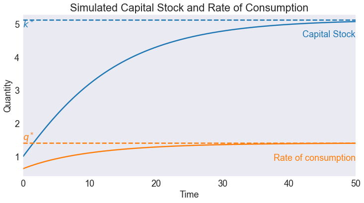
fig, ax = plt.subplots()
model.simulate([k0], T).plot(ax=ax)
ax.set(title='Simulated Capital Stock and Rate of Consumption',
       xlabel='Time',
       ylabel='Quantity',
       xlim=[0, T])

ax.axhline(kstar, ls='--', c='C0')
ax.axhline(qstar, ls='--', c='C1')

ax.annotate('$k^*$', (0, kstar), color='C0', va='top')
ax.annotate('$q^*$', (0, qstar), color='C1', va='bottom')

ax.annotate('\nCapital Stock', (T, kstar), color='C0', ha='right', va='top')
ax.annotate('\nRate of consumption', (T, qstar), color='C1', ha='right', va='top')

ax.legend([]);
PARAMETER xnames NO LONGER VALID. SET labels= AT OBJECT CREATION