KKT conditions for constrained optimization problems
KKT conditions for constrained optimization problems
Randall Romero Aguilar, PhD
This demo is based on the original Matlab demo accompanying the Computational Economics and Finance 2001 textbook by Mario Miranda and Paul Fackler.
Original (Matlab) CompEcon file: demopt06.m
Running this file requires the Python version of CompEcon. This can be installed with pip by running
!pip install compecon --upgrade
Last updated: 2021-Oct-01
import numpy as np
import matplotlib.pyplot as plt
from compecon.demos import demo

plt.style.use('seaborn')
%matplotlib inline
x = np.linspace(-0.5,1.5, 100)
a, b = 0.1, 1.1
ylim = [0.5, 2]
options = dict(
xlabel='$x$',
ylabel='$f (x)$',
xlim=[a-0.05, b+0.05],
ylim=ylim,
xticks=[a, b],
xticklabels=['a', 'b'],
yticks=ylim,
yticklabels=['', '']
)
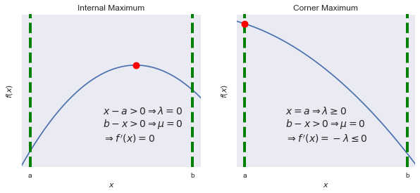
fig, (ax0, ax1) = plt.subplots(1,2,figsize=[10,4])
f = lambda x: 1.5 - 2*(x-0.75)**2
ax0.set(title='Internal Maximum', **options)
ax0.plot(x, f(x))
ax0.plot([a, a], ylim,'g--',linewidth=4)
ax0.plot([b, b], ylim,'g--',linewidth=4)
xstar = 0.75
ystar = f(xstar)
ax0.plot(xstar,ystar,'ro',ms=10)
ax0.annotate("$x-a>0\Rightarrow\lambda=0$\n$b-x>0\Rightarrow\mu=0$\n$\Rightarrow f\,'(x)=0$", (0.55,0.75),fontsize=14)
g = lambda x: 2 - 0.75*(x + 0.25)**2
ax1.set(title='Corner Maximum', **options)
ax1.plot(x, g(x))
ax1.plot([a, a], ylim,'g--',linewidth=4)
ax1.plot([b, b], ylim,'g--',linewidth=4)
ax1.plot(a,g(a),'ro',ms=10)
ax1.annotate("$x=a\Rightarrow\lambda\geq0$\n$b-x>0\Rightarrow\mu=0$\n$\Rightarrow f\,'(x)=-\lambda\leq0$", (0.35,0.75), fontsize=14);