Area under normal pdf using Simpson’s rule
Contents
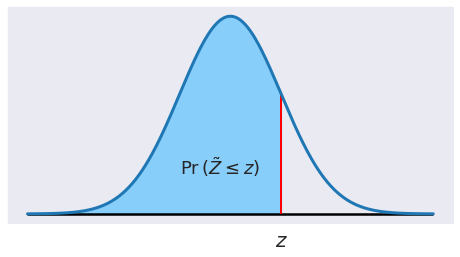
Area under normal pdf using Simpson’s rule
Randall Romero Aguilar, PhD
This demo is based on the original Matlab demo accompanying the Computational Economics and Finance 2001 textbook by Mario Miranda and Paul Fackler.
Original (Matlab) CompEcon file: demqua04.m
Running this file requires the Python version of CompEcon. This can be installed with pip by running
!pip install compecon --upgrade
Last updated: 2022-Oct-23
Initial tasks
import numpy as np
from compecon import qnwsimp
import matplotlib.pyplot as plt
n, a, z = 11, 0, 1

def f(x):
    return np.sqrt(1/(2*np.pi))*np.exp(-0.5*x**2)
x, w = qnwsimp(n, a, z)
prob = 0.5 + w.dot(f(x))
a, b, n = -4, 4, 500
x = np.linspace(a, b, n)
xz = np.linspace(a, z, n)

fig, ax = plt.subplots(figsize=[8,4])
ax.fill_between(xz,f(xz), color='LightSkyBlue')
ax.hlines(0, a, b,'k','solid')
ax.vlines(z, 0, f(z),'r',linewidth=2)
ax.plot(x,f(x), linewidth=3)

ax.annotate(r'$\Pr\left(\tilde Z\leq z\right)$',[-1, 0.08], fontsize=18)
ax.set_yticks([])
ax.set_xticks([z])
ax.set_xticklabels(['$z$'],fontsize=20);