Cournot Equilibrium Model
Contents
Cournot Equilibrium Model
Randall Romero Aguilar, PhD
This demo is based on the original Matlab demo accompanying the Computational Economics and Finance 2001 textbook by Mario Miranda and Paul Fackler.
Original (Matlab) CompEcon file: demslv05.m
Running this file requires the Python version of CompEcon. This can be installed with pip by running
!pip install compecon --upgrade
Last updated: 2022-Sept-04
There are two firms producing same good
Total cost of producing \(q_i\) in firm \(i\):
Inverse demand function:
Firm \(i\)’s profits:
Marginal profit for firm \(i\):
Therefore, equilibrium is characterized by solution to
The Jacobian matrix for this function is
Define
where \(\odot\) denotes the Hadamard (element-by-element) product of two matrices.
Then we can rewrite the \(f\) function and its Jacobian matrix as:
import numpy as np
import matplotlib.pyplot as plt
from compecon import NLP, gridmake
Parameters and initial value
alpha = 0.625
beta = np.array([0.6, 0.8])
Set up the Cournot function
def market(q):
    quantity = q.sum()
    price = quantity ** (-alpha)
    return price, quantity
def cournot(q):
    P, Q = market(q)
    P1 = -alpha * P/Q
    P2 = (-alpha - 1) * P1 / Q
    fval = P + (P1 - beta) * q
    fjac = np.diag(2 * P1 + P2 * q - beta) + np.fliplr(np.diag(P1 + P2 * q))
    return fval, fjac
We could also write the function and its Jacobian matrix more explicitly:
def cournot(q):
    P, Q = market(q)
    P1 = -alpha * P/Q
    P2 = (-alpha - 1) * P1 / Q
    fval = [P + (P1 - beta[0]) * q[0], P + (P1 - beta[0]) * q[0]]
    fjac = [[2 * P1 + P2 * q[0] - beta[0], P1 + P2 * q[0]],
            [P1 + P2 * q[1], 2 * P1 + P2 * q[1] - beta[1]]]
    return fval, fjac
However, the way it was defined earlier, in terms of matrix operations, is more convenient if we were to change the number of firms.
Compute equilibrium using Newton method (explicitly)
q = np.array([0.2, 0.2])

for it in range(40):
    f, J = cournot(q)
    step = -np.linalg.solve(J, f)
    q += step
    if np.linalg.norm(step) < 1.e-10: break

price, quantity = market(q)
print(f'Company 1 produces {q[0]:.4f} units, while company 2 produces {q[1]:.4f} units.')
print(f'Total production is {quantity:.4f} and price is {price:.4f}')
Company 1 produces 0.8396 units, while company 2 produces 0.6888 units.
Total production is 1.5284 and price is 0.7671
Using a NLP object
q0 = [0.2, 0.2]
cournot_problem = NLP(cournot)
q = cournot_problem.newton(q0, show=True)

price, quantity = market(q)
print(f'\nCompany 1 produces {q[0]:.4f} units, while company 2 produces {q[1]:.4f} units.')
print(f'Total production is {quantity:.4f} and price is {price:.4f}')
Solving nonlinear equations by Newton's method
it    bstep  change
--------------------
   0     0  4.64e-01
   1     0  9.53e-02
   2     0  3.47e-03
   3     0  4.20e-06
   4     0  5.77e-12

Company 1 produces 0.8396 units, while company 2 produces 0.6888 units.
Total production is 1.5284 and price is 0.7671
Generate data for contour plot
n = 100
q1 = np.linspace(0.1, 1.5, n)
q2 = np.linspace(0.1, 1.5, n)
z = np.array([cournot(q)[0] for q in gridmake(q1, q2).T]).T
Plot figures
steps_options = {'marker': 'o',
'color': (0.2, 0.2, .81),
'linewidth': 1.0,
'markersize': 9,
'markerfacecolor': 'white',
'markeredgecolor': 'red'}
contour_options = {'levels': [0.0],
'colors': '0.25',
'linewidths': 0.5}
Q1, Q2 = np.meshgrid(q1, q2)
Z0 = np.reshape(z[0], (n,n), order='F')
Z1 = np.reshape(z[1], (n,n), order='F')
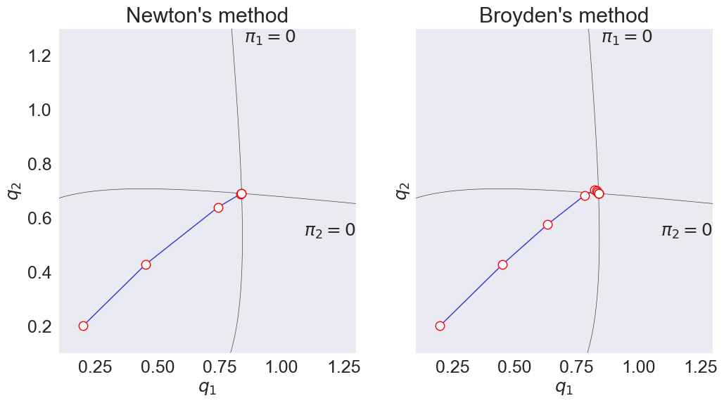
methods = ['newton', 'broyden']
cournot_problem.opts['maxit', 'maxsteps', 'all_x'] = 10, 0, True
qmin, qmax = 0.1, 1.3
fig, axs = plt.subplots(1,2,figsize=[12,6], sharey=True)
for ax, method in zip(axs, methods):
x = cournot_problem.zero(method=method)
ax.set(title=method.capitalize() + "'s method",
xlabel='$q_1$',
ylabel='$q_2$',
xlim=[qmin, qmax],
ylim=[qmin, qmax])
ax.contour(Q1, Q2, Z0, **contour_options)
ax.contour(Q1, Q2, Z1, **contour_options)
ax.plot(cournot_problem.x_sequence['x_0'], cournot_problem.x_sequence['x_1'], **steps_options)
ax.annotate('$\pi_1 = 0$', (0.85, qmax), ha='left', va='top')
ax.annotate('$\pi_2 = 0$', (qmax, 0.55), ha='right', va='center')
Solving nonlinear equations by Newton's method
it    bstep  change
--------------------
   0     0  1.10e+00
   1     0  4.64e-01
   2     0  9.53e-02
   3     0  3.47e-03
   4     0  4.20e-06
Solving nonlinear equations by Broyden's method
it    bstep  change
--------------------
   0     0  4.64e-01
   1     0  2.17e-01
   2     0  5.45e-02
   3     0  1.53e-02
   4     0  1.04e-02
   5     0  4.55e-03
   6     0  1.33e-04
   7     0  2.94e-07
   8     0  1.34e-09