Timber Harvesting Model - Cubic Spline Approximation
Contents
Timber Harvesting Model - Cubic Spline Approximation
Randall Romero Aguilar, PhD
This demo is based on the original Matlab demo accompanying the Computational Economics and Finance 2001 textbook by Mario Miranda and Paul Fackler.
Original (Matlab) CompEcon file: demdp01.m
Running this file requires the Python version of CompEcon. This can be installed with pip by running
!pip install compecon --upgrade
Last updated: 2022-Oct-22
About
Profit maximizing owner of a commercial tree stand must decide when to clearcut the stand.
import numpy as np
import matplotlib.pyplot as plt
import matplotlib.gridspec as gridspec
from compecon import DPmodel, BasisSpline, NLP
Model Parameters
Assuming that the unit price of biomass is \(p=1\), the cost to clearcut-replant is \(\kappa=0.2\), the stand carrying capacity \(s_{\max}=0.5\), biomass growth factor is \(\gamma=10\%\) per period, and the annual discount factor \(\delta=0.9\).
price = 1.0
κ = 0.2
smax  = 0.5
ɣ = 0.1
δ = 0.9
State Space
The state variable is the stand biomass, \(s\in [0,s_{\max}]\).
Here, we represent it with a cubic spline basis, with \(n=200\) nodes.
n = 200
basis = BasisSpline(n, 0, smax, labels=['biomass'])
Action Space
The action variable is \(j\in\{0:\text{'keep'},\quad 1:\text{'clear cut'}\}\).
options = ['keep', 'clear-cut']
Reward function
If the farmer clears the stand, the profit is the value of selling the biomass \(ps\) minus the cost of clearing and replanting \(\kappa\), otherwise the profit is zero.
def reward(s, x, i , j):
    return (price * s - κ) * j
State Transition Function
If the farmer clears the stand, it begins next period with \(\gamma s_{\max}\) units. If he keeps the stand, then it grows to \(s + \gamma (s_{\max} - s)\).
def transition(s, x, i, j, in_, e):
    if j:
        return np.full_like(s, ɣ * smax)
    else:
        return s + ɣ * (smax - s)
Model Structure
The value of the stand, given that it contains \(s\) units of biomass at the beginning of the period, satisfies the Bellman equation
To solve and simulate this model, use the CompEcon class DPmodel.
model = DPmodel(basis, reward, transition,
                discount=δ,
                j=options)

S = model.solve()
Solving infinite-horizon model collocation equation by Newton's method
iter change       time
------------------------------
   0       3.1e-01    0.0155
   1       1.1e-01    0.0155
   2       1.1e-02    0.0155
   3       4.6e-03    0.0311
   4       1.6e-16    0.0311
Elapsed Time =    0.03 Seconds
The solve method retuns a pandas DataFrame, which can easily be used to make plots. To see the first 10 entries of S, we use the head method
S.head()
| biomass | value | resid | j* | value[keep] | value[clear-cut] | |
|---|---|---|---|---|---|---|
| biomass | ||||||
| 0.000000 | 0.000000 | 0.067287 | -1.387779e-17 | keep | 0.067287 | -0.132713 |
| 0.000250 | 0.000250 | 0.067320 | -7.491474e-09 | keep | 0.067320 | -0.132462 |
| 0.000500 | 0.000500 | 0.067353 | -5.953236e-09 | keep | 0.067353 | -0.132212 |
| 0.000750 | 0.000750 | 0.067387 | -1.332984e-09 | keep | 0.067387 | -0.131962 |
| 0.001001 | 0.001001 | 0.067420 | 7.309628e-10 | keep | 0.067420 | -0.131712 |
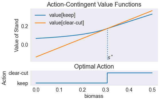
Analysis
To find the biomass level at which it is indifferent to keep or to clear cut, we interpolate as follows:
scrit = NLP(lambda s: model.Value_j(s).dot([1,-1])).broyden(0.0)
vcrit = model.Value(scrit)
print(f'When the biomass is {scrit:.5f} its value is {vcrit:.5f} regardless of the action taken by the manager')
When the biomass is 0.30669 its value is 0.17402 regardless of the action taken by the manager
Plot the Value Function and Optimal Action
?plt.subplots
fig1, axs = plt.subplots(2,1,figsize=[8,5], gridspec_kw=dict(height_ratios=[3.5, 1]))

S[['value[keep]', 'value[clear-cut]']].plot(ax=axs[0])
axs[0].set(title='Action-Contingent Value Functions',
           xlabel='',
           ylabel='Value of Stand',
           xticks=[])


ymin,ymax = axs[0].get_ylim()
axs[0].vlines(scrit,ymin, vcrit, linestyle=':')
axs[0].annotate('$s^*$', [scrit, ymin])

S['j*'].cat.codes.plot(ax=axs[1])
axs[1].set(title='Optimal Action',
           ylabel='Action',
           ylim=[-0.25,1.25],
           yticks=[0,1],
           yticklabels=options);
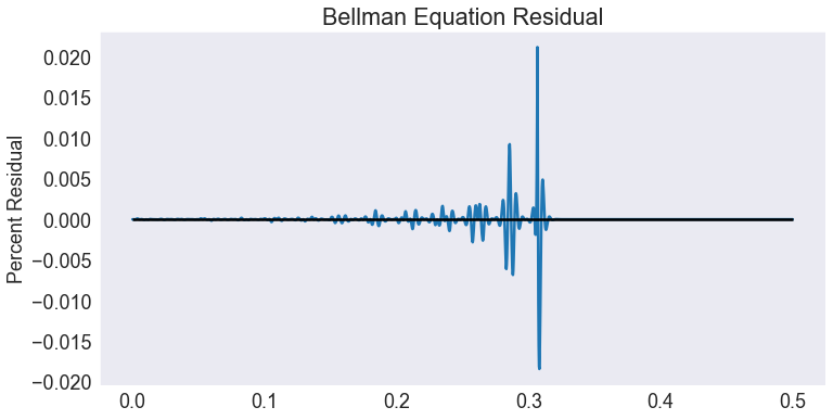
Plot Residuals
S['resid2'] = 100*S.resid / S.value

fig2, ax = plt.subplots()

ax.plot(S['resid2'])
ax.set(title='Bellman Equation Residual',
       xlabel='',
       ylabel='Percent Residual')

ax.hlines(0,0,smax,'k');
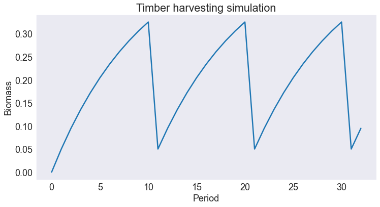
Simulation
The path followed by the biomass is computed by the simulate() method. Here we simulate 32 periods starting with a biomass level \(s_0 = 0\).
H = model.simulate(32, 0.0)

fig3, ax = plt.subplots()
ax.plot(H['biomass'])

ax.set(title='Timber harvesting simulation',
       xlabel='Period',
       ylabel='Biomass');