Inverse Demand Problem
Inverse Demand Problem
Randall Romero Aguilar, PhD
This demo is based on the original Matlab demo accompanying the Computational Economics and Finance 2001 textbook by Mario Miranda and Paul Fackler.
Original (Matlab) CompEcon file: demintro01.m
Running this file requires the Python version of CompEcon. This can be installed with pip by running
!pip install compecon --upgrade
Last updated: 2022-Ago-19
import numpy as np
import matplotlib.pyplot as plt
plt.style.use('seaborn-dark')
plt.style.use('seaborn-talk') # bigger fonts
demand = lambda p: 0.5 * p ** -0.2 + 0.5 * p ** -0.5
derivative = lambda p: -0.01 * p ** -1.2 - 0.25 * p ** -1.5


print('%12s %8s' % ('Iteration', 'Price'))
p = 0.25
for it in range(100):
    f = demand(p) - 2
    d = derivative(p)
    s = -f / d
    p += s
    print(f'{it:10d}   {p:8.4f}')
    if np.linalg.norm(s) < 1.0e-8:
        break

pstar = p
qstar = demand(pstar)
print(f'The equilibrium price is {pstar:.3f}, where demand is {qstar:.2f}')
   Iteration    Price
         0     0.0843
         1     0.1363
         2     0.1558
         3     0.1539
         4     0.1543
         5     0.1542
         6     0.1542
         7     0.1542
         8     0.1542
         9     0.1542
        10     0.1542
        11     0.1542
The equilibrium price is 0.154, where demand is 2.00
# Generate demand function
n, a, b = 100, 0.02, 0.40
p = np.linspace(a, b, n)
q = demand(p)

# Graph demand function
fig1, (ax0, ax1) = plt.subplots(1, 2, figsize=[12,6])
ax0.plot(p, q)

ax0.set(title='Demand',
        aspect=0.1,
        xlabel='price',
        xticks=[0.0, 0.2, 0.4],
        xlim=[0, 0.4],
        ylabel='quantity',
        yticks=[0, 2, 4],
        ylim=[0, 4])

# Graph inverse demand function
ax1.plot(q, p)
#ax1.plot([0, 2, 2], [pstar, pstar, 0], 'r--')
ax1.hlines(pstar, 0, 2, colors=['r'], linestyles=['--'])
ax1.vlines(2, 0, pstar, colors=['r'], linestyles=['--'])
ax1.plot([2], [pstar], 'ro', markersize=12)

ax1.set(title='Inverse Demand',
        aspect=10,
        xlabel='quantity',
        xticks=[0, 2, 4],
        xlim=[0, 4],
        ylabel='price',
        yticks=[0.0, pstar, 0.2, 0.4],
        yticklabels=['0.0', '$p^{*}$', '0.2', '0.4'],
        ylim=[0, 0.4]);
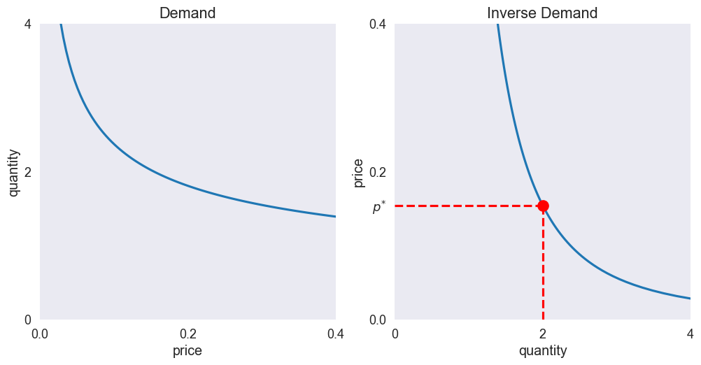
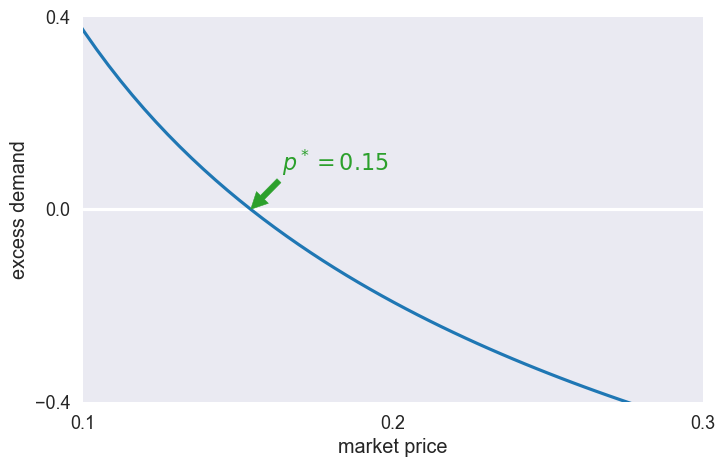
fig2, ax = plt.subplots(figsize=[8,5])
ax.axhline(0, color='w')
ax.plot(p, q-2)

ax.set(xlabel='market price',
       xticks=[0.1, 0.2, 0.3],
       xlim=[0.1, 0.3],
       ylabel='excess demand',
       yticks=[-0.4, 0, 0.4],
       ylim=[-0.4, 0.4])

ax.annotate(f'$p^*={pstar:.2f}$',
            (pstar, 0),
            (pstar+0.01, 0.08),
            color='C2',
            fontsize=16,
            arrowprops=dict(edgecolor='C2', facecolor='C2'));