Water Resource Management Model

Water Resource Management Model¶

Randall Romero Aguilar, PhD

This demo is based on the original Matlab demo accompanying the Computational Economics and Finance 2001 textbook by Mario Miranda and Paul Fackler.

Original (Matlab) CompEcon file: demdp01.m

Running this file requires the Python version of CompEcon. This can be installed with pip by running

!pip install compecon --upgrade

Last updated: 2022-Oct-23

About¶

Public authority must decide how much water to release from a reservoir so as to maximize benefits derived from agricultural and recreational uses.

States

s       reservoiur level at beginning of summer

Actions

x       quantity of water released for irrigation

Parameters
- a0,a1 – producer benefit function parameters
- b0,b1 – recreational user benefit function parameters
- \(\mu\) – mean rainfall
- \(\sigma\) – rainfall volatility
- \(\delta\) – discount factor

import numpy as np
import matplotlib.pyplot as plt
from compecon import BasisChebyshev, DPmodel, DPoptions, qnwlogn
import seaborn as sns
import pandas as pd

Model parameters¶

a0, a1, b0, b1 = 1, -2, 2, -3 
μ, σ, δ = 1.0, 0.2, 0.9

Steady-state¶

The deterministic steady-state values for this model are

xstar = 1.0  # action
sstar = 1.0 + (a0*(1-δ)/b0)**(1/b1)  # stock

State space¶

The state variable is s=”Reservoir Level”, which we restrict to \(s\in[2, 8]\).

Here, we represent it with a Chebyshev basis, with \(n=15\) nodes.

n, smin, smax = 15, 2, 8
basis = BasisChebyshev(n, smin, smax, labels=['Reservoir'])

Continuous state shock distribution¶

m = 3  #number of rainfall shocks
e, w = qnwlogn(m, np.log(μ)-σ**2/2,σ**2) # rainfall shocks and proabilities

Action space¶

The choice variable x=”Irrigation” must be nonnegative.

def bounds(s, i=None, j=None):
    return np.zeros_like(s), 1.0*s

Reward function¶

The reward function is

def reward(s, x, i=None, j=None):
    sx = s-x
    u = (a0/(1+a1))*x**(1+a1) + (b0/(1+b1))*sx**(1+b1)
    ux = a0*x**a1 - b0*sx**b1                                 
    uxx = a0*a1*x**(a1-1) + b0*b1*sx**(b1-1)  
    return u, ux, uxx

State transition function¶

Next period, reservoir level wealth will be equal to current level minus irrigation plus random rainfall:

def transition(s, x, i=None, j=None, in_=None, e=None):
    g = s - x + e
    gx = -np.ones_like(s)
    gxx = np.zeros_like(s)
    return g, gx, gxx

Model structure¶

The value of wealth \(s\) satisfies the Bellman equation

\[\begin{equation*} V(s) = \max_x\left\{\left(\frac{a_0}{1+a_1}\right)x^{1+a1} + \left(\frac{b_0}{1+b_1}\right)(s-x)^{1+b1}+ \delta V(s-x+e) \right\} \end{equation*}\]

To solve and simulate this model,use the CompEcon class DPmodel

water_model = DPmodel(basis, reward, transition, bounds,e=e,w=w,
                       x=['Irrigation'],
                       discount=δ )

Solving the model¶

Compute Linear-Quadratic Approximation at Collocation Nodes¶

The DPmodel.lqapprox solves the linear-quadratic approximation, in this case arround the steady-state. It returns a LQmodel which works similar to the DPmodel object. We compute the solution at the basis nodes to use it as initial guess for the Newton’s methods.

water_lq = water_model.lqapprox(sstar,xstar).solution(basis.nodes)

Solving the growth model by collocation. We take the values for the Value and Policy functions at the basis nodes obtained from the linear-quadratic approximation as initial guess values for the Newton’s method.

S = water_model.solve(v=water_lq['value'], x=water_lq['Irrigation'])
S.head()

Solving infinite-horizon model collocation equation by Newton's method
iter change       time    
------------------------------
   0       7.1e-01    0.0156
   1       1.2e-01    0.0156
   2       1.2e-02    0.0312
   3       1.3e-04    0.0312
   4       1.9e-08    0.0468
   5       4.6e-15    0.0468
Elapsed Time =    0.05 Seconds

	Reservoir	value	resid	Irrigation
Reservoir
2.000000	2.000000	-14.086357	8.445569e-07	0.628126
2.040268	2.040268	-13.985981	-6.417778e-07	0.638659
2.080537	2.080537	-13.888843	-7.616363e-07	0.649069
2.120805	2.120805	-13.794753	-3.379168e-07	0.659357
2.161074	2.161074	-13.703538	1.731421e-07	0.669527

DPmodel.solve returns a pandas DataFrame with the following data:

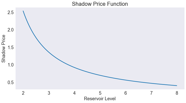
We are also interested in the shadow price of wealth (the first derivative of the value function).

S['shadow price'] = water_model.Value(S['Reservoir'],1)
S.head()

	Reservoir	value	resid	Irrigation	shadow price
Reservoir
2.000000	2.000000	-14.086357	8.445569e-07	0.628126	2.534519
2.040268	2.040268	-13.985981	-6.417778e-07	0.638659	2.451652
2.080537	2.080537	-13.888843	-7.616363e-07	0.649069	2.373665
2.120805	2.120805	-13.794753	-3.379168e-07	0.659357	2.300174
2.161074	2.161074	-13.703538	1.731421e-07	0.669527	2.230828

Plotting the results¶

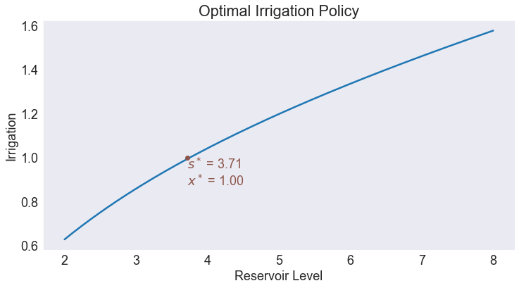
Optimal Policy¶

fig1, ax = plt.subplots()
ax.set(title='Optimal Irrigation Policy', xlabel='Reservoir Level', ylabel='Irrigation')
ax.plot(S['Irrigation'])

ax.plot(sstar, xstar, 'o', color='C5');
ax.annotate(f'$s^*$ = {sstar:.2f}\n$x^*$ = {xstar:.2f}', [sstar, xstar], va='top', color='C5');

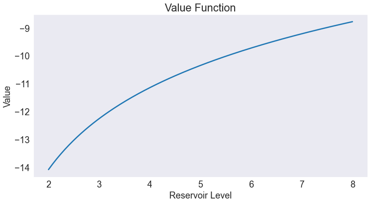
../../_images/10 Water Resource Management Model_29_0.png

Value Function¶

fig2, ax = plt.subplots()
ax.set(title='Value Function', xlabel='Reservoir Level', ylabel='Value')
ax.plot(S['value']);

../../_images/10 Water Resource Management Model_31_0.png

Shadow Price Function¶

fig3, ax = plt.subplots()
ax.set(title='Shadow Price Function', xlabel='Reservoir Level', ylabel='Shadow Price')
ax.plot(S['shadow price']);

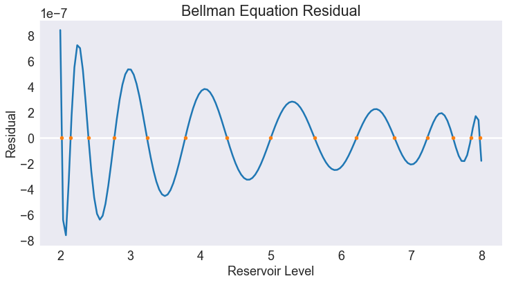
../../_images/10 Water Resource Management Model_33_0.png

Chebychev Collocation Residual¶

fig4, ax = plt.subplots()
ax.set(title='Bellman Equation Residual', xlabel='Reservoir Level', ylabel='Residual')
ax.axhline(0, color='w')
ax.plot(S['resid'])
ax.plot(basis.nodes[0], np.zeros_like(basis.nodes[0]), lw=0, marker='.', markersize=9)
ax.ticklabel_format(style='sci', axis='y', scilimits=(-1,1))

../../_images/10 Water Resource Management Model_35_0.png

Simulating the model¶

We simulate 21 periods of the model starting from \(s=s_{\min}\)

T = 31
nrep = 100_000
data = water_model.simulate(T, np.tile(smin,nrep))

Simulated State and Policy Paths¶

subdata = data.query('_rep < 100')

fig6, ax = plt.subplots()
ax.set(title='Simulated and Expected Reservoir Level', 
       xlabel='Year', 
       ylabel='Reservoir Level',
       xlim=[0, T + 0.5])

ax.plot(data[['time','Reservoir']].groupby('time').mean())
ax.plot(subdata.pivot('time','_rep','Reservoir'),lw=1, color='C0', alpha=0.2)

ax.annotate(f'steady-state reservoir\n = {sstar:.2f}',[T, sstar], color='C0', ha='right', va='top')

Text(31, 3.7144176165949068, 'steady-state reservoir\n = 3.71')

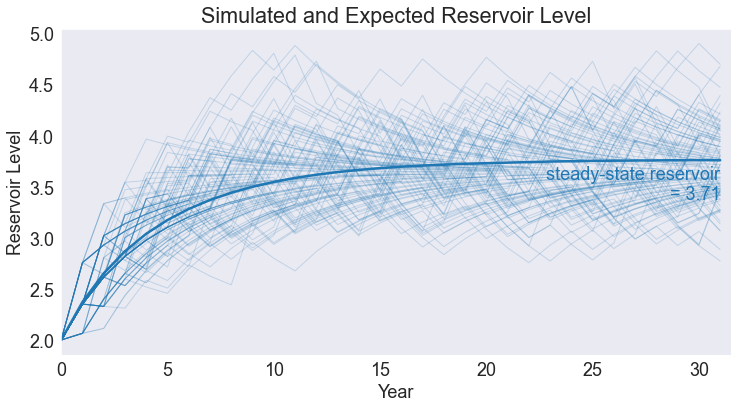
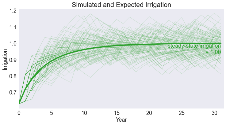
../../_images/10 Water Resource Management Model_40_1.png

fig7, ax = plt.subplots()
ax.set(title='Simulated and Expected Irrigation', 
       xlabel='Year', 
       ylabel='Irrigation',
       xlim=[0, T + 0.5])

ax.plot(subdata.pivot('time','_rep','Irrigation'),lw=1, color='C2', alpha=0.2)
ax.plot(data[['time','Irrigation']].groupby('time').mean(), color='C2', lw=4)

ax.annotate(f'steady-state irrigation\n = {xstar:.2f}',[T, xstar], color='C2', ha='right', va='top')

Text(31, 1.0, 'steady-state irrigation\n = 1.00')

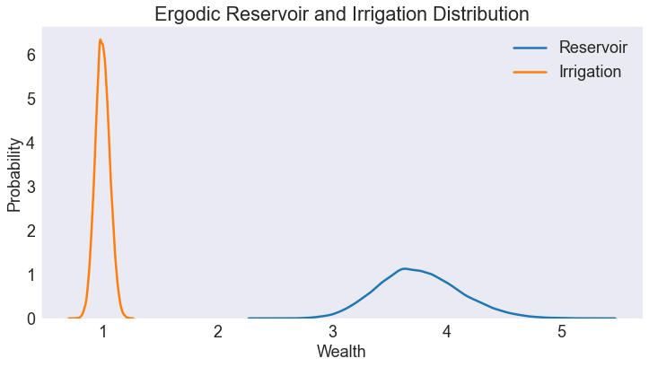
../../_images/10 Water Resource Management Model_41_1.png

Ergodic Wealth Distribution¶

subdata = data[data['time']==T][['Reservoir','Irrigation']]
stats =pd.DataFrame({'Deterministic Steady-State': [sstar, xstar],
              'Ergodic Means': subdata.mean(),
              'Ergodic Standard Deviations': subdata.std()}).T
stats

	Reservoir	Irrigation
Deterministic Steady-State	3.714418	1.000000
Ergodic Means	3.761570	0.999193
Ergodic Standard Deviations	0.358572	0.062345

fig8, ax = plt.subplots()
ax.set(title='Ergodic Reservoir and Irrigation Distribution',xlabel='Wealth',ylabel='Probability')
sns.kdeplot(subdata['Reservoir'], ax=ax, label='Reservoir')
sns.kdeplot(subdata['Irrigation'], ax=ax, label='Irrigation')
ax.legend();

../../_images/10 Water Resource Management Model_44_0.png

Private Non-Renewable Resource Model

Monetary Policy Model

A Python Implementation of CompEcon