Stability of Linear Homogeneous ODEs
Contents
Stability of Linear Homogeneous ODEs
Randall Romero Aguilar, PhD
This demo is based on the original Matlab demo accompanying the Computational Economics and Finance 2001 textbook by Mario Miranda and Paul Fackler.
Original (Matlab) CompEcon file: demode01.m
Running this file requires the Python version of CompEcon. This can be installed with pip by running
!pip install compecon --upgrade
Last updated: 2021-Oct-01
This demo is hard to run, because it requieres user to install ffmpeg
from compecon import ODE

import numpy as np
import pandas as pd
import matplotlib.pyplot as plt

ANIMATED = 3 # static images if 0, videos of ANIMATED seconds if positive. Requires ffmpeg
def annotate_line(ax, str, l, pos=0.1, **kwargs):

    xlim=ax.get_xlim()
    ylim=ax.get_ylim()

    x=np.asarray(l.get_xdata())
    y=np.asarray(l.get_ydata())

    dx = x[1] - x[0]
    dy = y[1] - y[0]
    angle = np.arctan(dy/dx)*180/np.pi if dx else 90

    is_visible = (x >=xlim[0]) & (x<=xlim[1]) & (y >=ylim[0]) & (y<=ylim[1])
    x = x[is_visible]
    y = y[is_visible]

    xt = pos * x[-1] + (1-pos)*x[0]
    yt = pos * y[-1] + (1-pos)*y[0]

    ax.annotate(str, (xt,yt), rotation=angle, ha="center", **kwargs)


def phase(A,figtitle, stable=True, pos=(0.1,0.1)):
    xlim = [-1.05, 1.05]

    A = np.asarray(A)

    problems = [ODE(lambda x: A @ x, T=T,bv=bv) for bv in x0]

    for problem in problems:
        problem.solve_collocation()


    fig, ax = plt.subplots(figsize=[8,8])
    ax.set_aspect('equal', adjustable='box')

    # Compute and plot Nullclines
    xnulls_kw=dict(ls="--", color="gray")
    x1 = np.linspace(*xlim, 100)

    if A[0,1]:
        lx0, = ax.plot(x1, -(A[0,0]*x1)/A[0,1], **xnulls_kw)
    else:
        lx0, = ax.plot([0,0], xlim, **xnulls_kw)

    if A[1,1]:
        lx1, = ax.plot(x1, -(A[1,0]*x1)/A[1,1], **xnulls_kw)
    else:
        lx1, = ax.plot([0,0], xlim, **xnulls_kw)

    annotate_line(ax, '$\dot{y}_{0}=0$', lx0, pos=pos[0], color=xnulls_kw['color'], fontsize=16)
    annotate_line(ax, '$\dot{y}_{1}=0$', lx1, pos=pos[1], color=xnulls_kw['color'], fontsize=16)


    # Eigenvalues
    D, V = np.linalg.eig(A);
    V = np.sqrt(2)*V

    print('Eigenvalues', D, sep='\n')
    print('\nEigenvectors', V, sep='\n')


    if np.isreal(D[0]):
        for j in range(2):
            color = 'darkseagreen' if D[j] < 0 else 'lightcoral'
            ax.plot([-V[0,j], V[0,j]], [-V[1,j], V[1,j]], color=color)
            ax.annotate(f'$v_{j}$', V[:,j], color=color, fontsize=14)

    video = problem.phase(xlim, xlim, ax=ax, animated=ANIMATED,
                          x=np.array([problem.x.values.T for problem in problems]),
                          title=figtitle,
                          path_kw=dict(color="forestgreen" if stable else "firebrick"),
                          xticks=[-1,0,1], yticks=[-1,0,1]
                         )


    return ax.figure, video
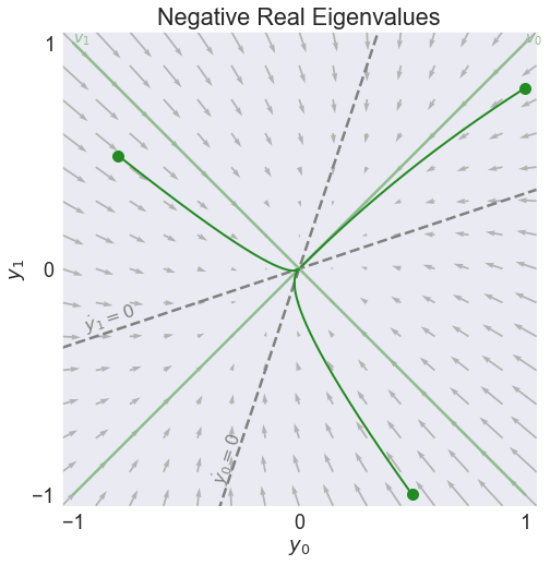
Example 1
A = [[-0.75, 0.25],[0.25, -0.75]]
x0 = [[1.0, 0.8], [-0.8, 0.5], [0.5, -1.0]]
T = 10
fig1, video1 = phase(A,'Negative Real Eigenvalues', stable=True, pos=[0.35,0.1])
video1
Eigenvalues
[-0.5 -1. ]

Eigenvectors
[[ 1. -1.]
 [ 1.  1.]]
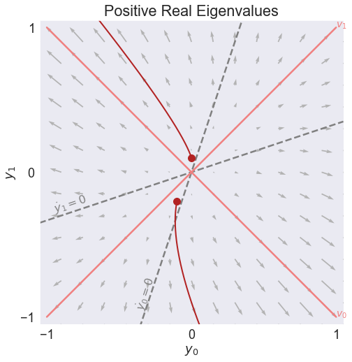
Example 2
A = [[0.75, -0.25],[-0.25, 0.75]]
x0 = [[-0.1, -0.2], [0, 0.1]]
T = 3
fig2, video2 = phase(A,'Positive Real Eigenvalues', stable=False, pos=[0.35,0.1])
video2
Eigenvalues
[1.  0.5]

Eigenvectors
[[ 1.  1.]
 [-1.  1.]]
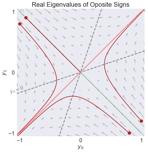
Example 3
A = [[-0.25, 0.75],[0.75, -0.25]]
x0 = [[1.0, -0.8], [-1,0.8],[0.8,-1], [-0.9,0.9]]
T = 5
fig3, video3 = phase(A,'Real Eigenvalues of Oposite Signs', stable=False, pos=[0,0.05])
video3
Eigenvalues
[ 0.5 -1. ]

Eigenvectors
[[ 1. -1.]
 [ 1.  1.]]
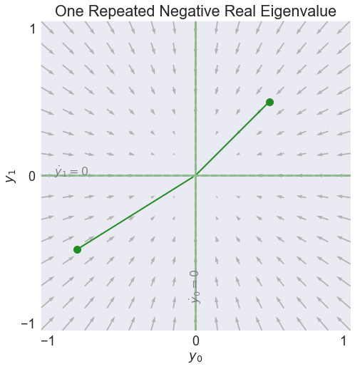
Example 4
A = [[-0.5, 0],[0, -0.5]]
x0 = [[0.5, 0.5], [-0.8,-0.5]]
T = 8
fig4, video4 = phase(A,'One Repeated Negative Real Eigenvalue', stable=True)
video4
Eigenvalues
[-0.5 -0.5]

Eigenvectors
[[1.4142 0.    ]
 [0.     1.4142]]
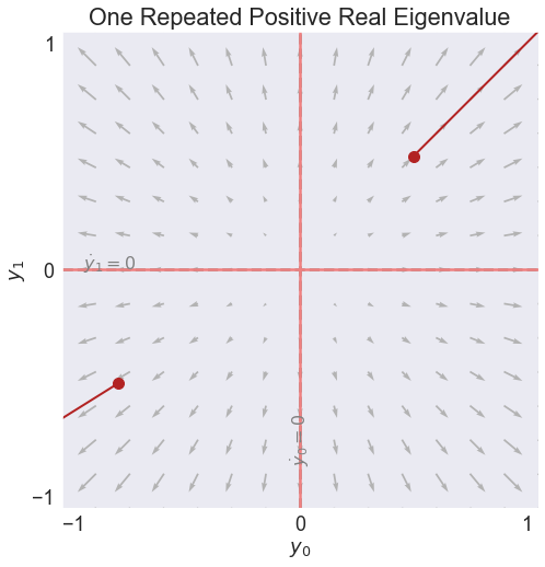
Example 5
A = [[0.5, 0],[0, 0.5]]
x0 = [[0.5, 0.5], [-0.8,-0.5]]
T = 2
fig5, video5 = phase(A,'One Repeated Positive Real Eigenvalue', stable=False)
video5
Eigenvalues
[0.5 0.5]

Eigenvectors
[[1.4142 0.    ]
 [0.     1.4142]]
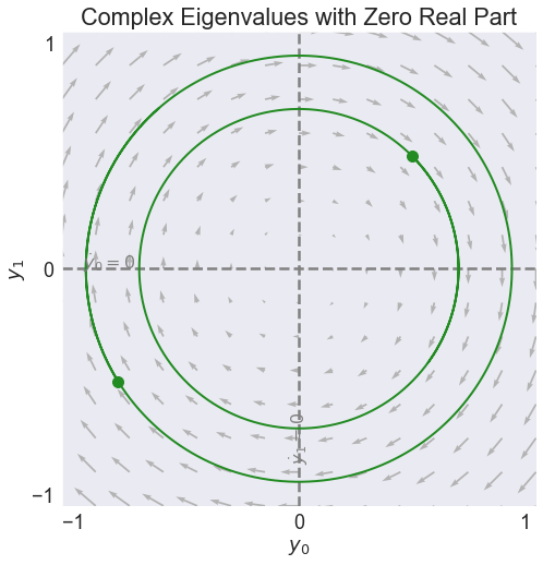
Example 6
A = [[0, 1],[-1, 0]]
x0 = [[0.5, 0.5], [-0.8,-0.5]]
T = 8
fig6, video6 = phase(A,'Complex Eigenvalues with Zero Real Part', stable=True)
video6
Eigenvalues
[0.+1.j 0.-1.j]

Eigenvectors
[[1.+0.j 1.+0.j]
 [0.+1.j 0.-1.j]]
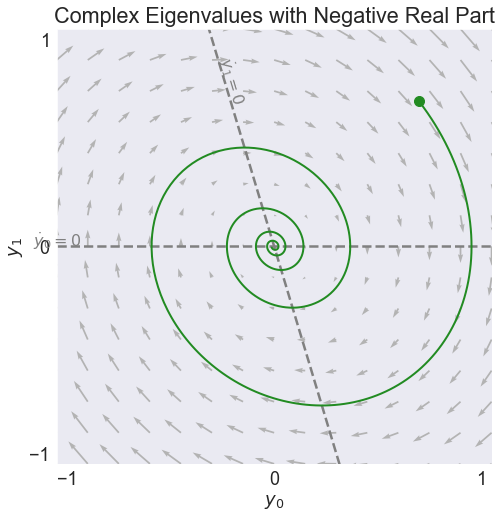
Example 7
A = [[0, 1],[-1, -0.3]]
x0 = [[0.7, 0.7]]
T = 30
fig7, video7 = phase(A,'Complex Eigenvalues with Negative Real Part', stable=True, pos=[0,0.4])
video7
Eigenvalues
[-0.15+0.9887j -0.15-0.9887j]

Eigenvectors
[[ 1.  +0.j      1.  +0.j    ]
 [-0.15+0.9887j -0.15-0.9887j]]
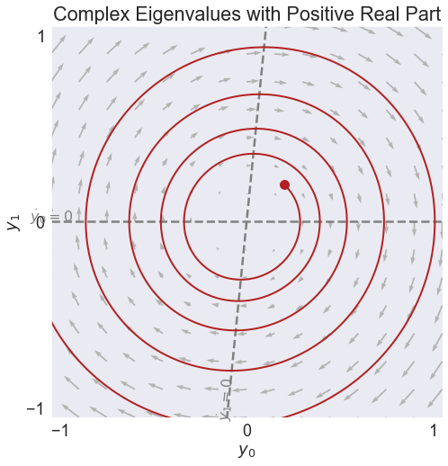
Example 8
A = [[0, 1], [-1, 0.1]]
x0 = [[0.2, 0.2]]
T = 30
fig8, video8 = phase(A,'Complex Eigenvalues with Positive Real Part', stable=False, pos=[0,0.45])
video8
Eigenvalues
[0.05+0.9987j 0.05-0.9987j]

Eigenvectors
[[1.  +0.j     1.  +0.j    ]
 [0.05+0.9987j 0.05-0.9987j]]
#for i, fig in enumerate([fig1, fig2, fig3, fig4, fig5, fig6, fig7, fig8], start=1):
#    fig.savefig(f'ode-example{i}.pdf', bbox_inches='tight')