Demonstrates accuracy of one- and two-sided finite-difference derivatives
Contents
Demonstrates accuracy of one- and two-sided finite-difference derivatives
Randall Romero Aguilar, PhD
This demo is based on the original Matlab demo accompanying the Computational Economics and Finance 2001 textbook by Mario Miranda and Paul Fackler.
Original (Matlab) CompEcon file: demdif02.m
Running this file requires the Python version of CompEcon. This can be installed with pip by running
!pip install compecon --upgrade
Last updated: 2022-Oct-22
About
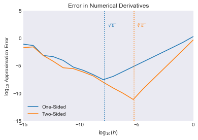
Demonstrates accuracy of one- and two-sided finite-difference derivatives of \(e^x\) at \(x=1\) as a function of step size \(h\).
Initial tasks
import numpy as np
import matplotlib.pyplot as plt
plt.style.use('seaborn-dark')
Setting parameters
n, x = 18, 1.0
c = np.linspace(-15,0,n)
h = 10 ** c
exp = np.exp
eps = np.finfo(float).eps

def deriv_error(l, u):
    dd = (exp(u) - exp(l)) / (u-l)
    return np.log10(np.abs(dd - exp(x)))
One-sided finite difference derivative
d1 = deriv_error(x, x+h)
e1 = np.log10(eps**(1/2))
Two-sided finite difference derivative
d2 = deriv_error(x-h, x+h)
e2 = np.log10(eps**(1/3))
Plot finite difference derivatives
fig, ax = plt.subplots()
ax.plot(c,d1, label='One-Sided')
ax.plot(c,d2, label='Two-Sided')
ax.axvline(e1, color='C0', linestyle=':')
ax.axvline(e2, color='C1',linestyle=':')

ax.set(title='Error in Numerical Derivatives',
       xlabel='$\log_{10}(h)$',
       ylabel='$\log_{10}$ Approximation Error',
       xlim=[-15, 0], xticks=np.arange(-15,5,5),
       ylim=[-15, 5], yticks=np.arange(-15,10,5)
       )

ax.annotate('$\sqrt{\epsilon}$', (e1+.25, 2), color='C0')
ax.annotate('$\sqrt[3]{\epsilon}$', (e2 +.25, 2),color='C1')
ax.legend(loc='lower left');