.ipynb .pdf

repository open issue

Binder Colab

Contents

Monetary Policy Model

Randall Romero Aguilar, PhD

This demo is based on the original Matlab demo accompanying the Computational Economics and Finance 2001 textbook by Mario Miranda and Paul Fackler.

Original (Matlab) CompEcon file: demdp11.m

Running this file requires the Python version of CompEcon. This can be installed with pip by running

!pip install compecon --upgrade

Last updated: 2022-Oct-23

---

About

A central bank must set nominal interest rate so as to minimize deviations of inflation rate and GDP gap from established targets.

A monetary authority wishes to control the nominal interest rate \(x\) in order to minimize the variation of the inflation rate \(s_1\) and the gross domestic product (GDP) gap \(s_2\) around specified targets \(s^∗_1\) and \(s^∗_2\), respectively. Specifically, the authority wishes to minimize expected discounted stream of weighted squared deviations

\[\begin{equation*} L(s) = \frac{1}{2}(s − s^∗)'\Omega(s − s^∗) \end{equation*}\]

where \(s\) is a \(2\times 1\) vector containing the inflation rate and the GDP gap, \(s^∗\) is a \(2\times 1\) vector of targets, and \(\Omega\) is a \(2 \times 2\) constant positive definite matrix of preference weights. The inflation rate and the GDP gap are a joint controlled exogenous linear Markov process

\[\begin{equation*} s_{t+1} = \alpha + \beta s_t + \gamma x_t + \epsilon_{t+1} \end{equation*}\]

where \(\alpha\) and \(\gamma\) are \(2 \times 1\) constant vectors, \(\beta\) is a \(2 \times 2\) constant matrix, and \(\epsilon\) is a \(2 \times 1\) random vector with mean zero. For institutional reasons, the nominal interest rate \(x\) cannot be negative. What monetary policy minimizes the sum of current and expected future losses?

This is an infinite horizon, stochastic model with time \(t\) measured in years. The state vector \(s \in \mathbb{R}^2\) contains the inflation rate and the GDP gap. The action variable \(x \in [0,\infty)\) is the nominal interest rate. The state transition function is \(g(s, x, \epsilon) = \alpha + \beta s + \gamma x + \epsilon\)

In order to formulate this problem as a maximization problem, one posits a reward function that equals the negative of the loss function \(f(s,x) = −L(s)\)

The sum of current and expected future rewards satisfies the Bellman equation

\[\begin{equation*} V(s) = \max_{0\leq x}\left\{-L(s) + \delta + E_\epsilon V\left(g(s,x,\epsilon)\right)\right\} \end{equation*}\]

Given the structure of the model, one cannot preclude the possibility that the nonnegativity constraint on the optimal nominal interest rate will be binding in certain states. Accordingly, the shadow-price function \(\lambda(s)\) is characterized by the Euler conditions

\[\begin{align*} \delta\gamma'E_\epsilon \lambda\left(g(s,x,\epsilon)\right) &= \mu \\ \lambda(s) &= -\Omega(s-s^*) + \delta\beta'E_\epsilon \lambda\left(g(s,x,\epsilon)\right) \end{align*}\]

where the nominal interest rate \(x\) and the long-run marginal reward \(\mu\) from increasing the nominal interest rate must satisfy the complementarity condition

\[\begin{equation*} x \geq 0, \qquad \mu \leq 0, \qquad x > 0 \Rightarrow \mu = 0 \end{equation*}\]

It follows that along the optimal path

\[\begin{align*} \delta\gamma'E_\epsilon \lambda_{t+1} &= \mu_t \\ \lambda_t &= -\Omega(s_t-s^*) + \delta\beta'E_\epsilon \lambda_{t+1}\\ x \geq 0, \qquad \mu \leq 0, &\qquad x > 0 \Rightarrow \mu = 0 \end{align*}\]

Thus, in any period, the nominal interest rate is reduced until either the long-run marginal reward or the nominal interest rate is driven to zero.

import numpy as np
import matplotlib.pyplot as plt
from mpl_toolkits.mplot3d import Axes3D
from matplotlib import cm
from compecon import BasisChebyshev, DPmodel, BasisSpline, qnwnorm
import pandas as pd
pd.set_option('display.float_format',lambda x: f'{x:.3f}')

Model Parameters

α   = np.array([[0.9, -0.1]]).T             # transition function constant coefficients
β    = np.array([[-0.5, 0.2], [0.3, -0.4]])  # transition function state coefficients
γ   = np.array([[-0.1, 0.0]]).T             # transition function action coefficients
Ω   = np.identity(2)                        # central banker's preference weights
ξ   = np.array([[1, 0]]).T                  # equilibrium targets
μ   = np.zeros(2)                           # shock mean
σ   = 0.08 * np.identity(2),                # shock covariance matrix
δ   = 0.9                                   # discount factor

State Space

There are two state variables: ‘GDP gap’ = \(s_0\in[-2,2]\) and ‘inflation’=\(s_1\in[-3,3]\).

n = 21          
smin = [-2, -3] 
smax = [ 2,  3] 

basis = BasisChebyshev(n, smin, smax, method='complete',
                       labels=['GDP gap', 'inflation'])

Action space

There is only one action variable x: the nominal interest rate, which must be nonnegative.

def bounds(s, i, j):
    lb  = np.zeros_like(s[0])
    ub  = np.full(lb.shape, np.inf)
    return lb, ub

Reward Function

def reward(s, x, i, j):
    s = s - ξ
    f = np.zeros_like(s[0])
    for ii in range(2):
        for jj in range(2):
            f -= 0.5 * Ω[ii, jj] * s[ii] * s[jj]
    fx = np.zeros_like(x)
    fxx = np.zeros_like(x)
    return f, fx, fxx

State Transition Function

def transition(s, x, i, j, in_, e):
    g = α + β @ s + γ @ x + e
    gx = np.tile(γ, (1, x.size))
    gxx = np.zeros_like(s)
    return g, gx, gxx

The continuous shock must be discretized. Here we use Gauss-Legendre quadrature to obtain nodes and weights defining a discrete distribution that matches the first 6 moments of the Normal distribution (this is achieved with m=3 nodes and weights) for each of the state variables.

m   = [3, 3]
[e,w] = qnwnorm(m,μ,σ)

Model structure

bank = DPmodel(basis, reward, transition, bounds,
               x=['interest'], discount=δ, e=e, w=w)

Compute Unconstrained Deterministic Steady-State

bank_lq = bank.lqapprox(ξ,0)

sstar = bank_lq.steady['s']
xstar = bank_lq.steady['x']

If Nonnegativity Constraint Violated, Re-Compute Deterministic Steady-State

if xstar < 0:
    I = np.identity(2)
    xstar = 0.0
    sstar = np.linalg.solve(np.identity(2) - β, α)

frmt = '\t%-21s = %5.2f' 
print('Deterministic Steady-State')
print(frmt % ('GDP Gap', sstar[0]))
print(frmt % ('Inflation Rate', sstar[1]))
print(frmt % ('Nominal Interest Rate', xstar))

Deterministic Steady-State
	GDP Gap               =  0.61
	Inflation Rate        =  0.06
	Nominal Interest Rate =  0.00

Solve the model

We solve the model by calling the solve method in bank. On return, sol is a pandas dataframe with columns GDP gap, inflation, value, interest, and resid. We set a refined grid nr=5 for this output.

S = bank.solve(nr=5)

Solving infinite-horizon model collocation equation by Newton's method
iter change       time    
------------------------------

   0       6.7e+00    0.2664

   1       9.9e-01    0.8448

   2       9.1e-04    1.4133

   3       8.3e-07    1.8668

   4       7.7e-09    2.3227
Elapsed Time =    2.32 Seconds

To make the 3D plots, we need to reshape the columns of sol.

S3d = {x: S[x].values.reshape((5*n,5*n)) for x in S.columns}

This function will make all plots

def makeplot(series,zlabel,zticks,title):
    fig = plt.figure(figsize=[12,6])
    ax = fig.gca(projection='3d')
    ax.plot_surface(S3d['GDP gap'], S3d['inflation'], S3d[series], cmap=cm.coolwarm)
    ax.set_xlabel('GDP gap')
    ax.set_ylabel('Inflation')
    ax.set_zlabel(zlabel)  
    ax.set_xticks(np.arange(-2,3))
    ax.set_yticks(np.arange(-3,4))
    ax.set_zticks(zticks)
    ax.set_title(title)
    return fig, ax

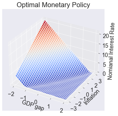
Optimal policy

fig1, ax = makeplot('interest', 'Nomianal Interest Rate',
               np.arange(0,21,5),'Optimal Monetary Policy')

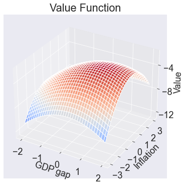
Value function

fig2, ax = makeplot('value','Value',
                np.arange(-12,S['value'].max(),4),'Value Function')

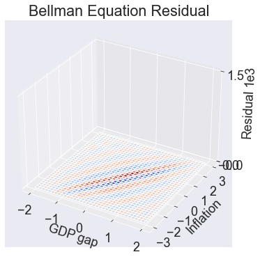
Residuals

fig3, ax = makeplot('resid','Residual',
                [-1.5e-3, 0, 1.5e3],'Bellman Equation Residual')
ax.ticklabel_format(style='sci', axis='z', scilimits=(-1,1))

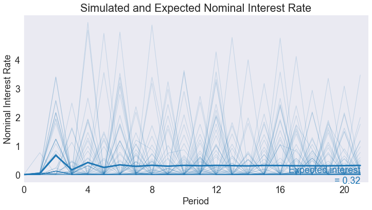
Simulating the model

We simulate 21 periods of the model starting from \(s=s_{\min}\), 10000 repetitions.

T = 21
nrep = 10_000
data = bank.simulate(T, np.tile(np.atleast_2d(smax).T,nrep))

subdata = data[data['time']==T][['GDP gap', 'inflation', 'interest']]
stats =pd.DataFrame({'Deterministic Steady-State': [*sstar.flatten(), xstar],
              'Ergodic Means': subdata.mean(),
              'Ergodic Standard Deviations': subdata.std()})
stats.T

	GDP gap	inflation	interest
Deterministic Steady-State	0.608	0.059	0.000
Ergodic Means	0.586	0.060	0.319
Ergodic Standard Deviations	0.318	0.336	0.726

Simulated State and Policy Paths

subdata = data.query('_rep < 60')
gdpstar, infstar, intstar = stats['Ergodic Means']

def simplot(series,ylabel,yticks,steady):
    fig, ax = plt.subplots()
    ax.set(title='Simulated and Expected ' + ylabel, 
           xlabel='Period', 
           ylabel=ylabel, 
           xlim=[0, T + 0.5], 
           xticks=range(0,T+1,4),
           yticks=yticks)
    ax.plot(data[['time',series]].groupby('time').mean(), lw=3)
    ax.plot(subdata.pivot('time','_rep',series),lw=1, alpha=0.2, color='C0')
    ax.annotate(f'Expected {series}\n = {steady:.2f}', [T, steady],  ha='right', va='top', color='C0')
    return fig

fig4 = simplot('GDP gap','GDP gap',np.arange(smin[0],smax[0]+1),gdpstar)

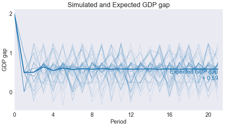
fig5 = simplot('inflation', 'Inflation Rate',np.arange(smin[1],smax[1]+1),infstar)

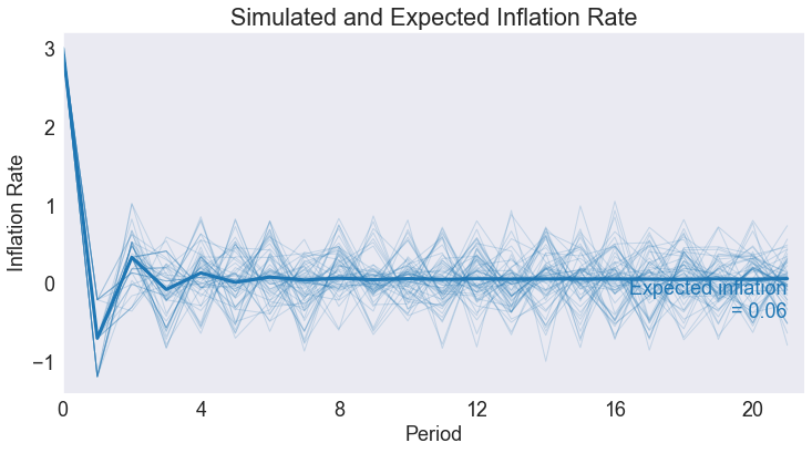
fig6 = simplot('interest','Nominal Interest Rate',np.arange(-2,5),intstar)

previous

Water Resource Management Model

next

Linear-Quadratic Model