Non-IVP Non-Homogeneous Linear ODE Example
Contents
Non-IVP Non-Homogeneous Linear ODE Example
Randall Romero Aguilar, PhD
This demo is based on the original Matlab demo accompanying the Computational Economics and Finance 2001 textbook by Mario Miranda and Paul Fackler.
Original (Matlab) CompEcon file: demode04.m
Running this file requires the Python version of CompEcon. This can be installed with pip by running
!pip install compecon --upgrade
Last updated: 2021-Oct-01
About
Solve
\[\begin{align*}
\dot{x_1} &= -1*x_1 - 0.5x_2 + 2\\
\dot{x_2} &= -0.5x_2 + 1
\end{align*}\]
subject to
\[\begin{align*}
x_1(0) &=1\\
x_2(1) &=1\\
t &\in [0, 10]
\end{align*}\]
FORMULATION
from compecon import jacobian, ODE

import numpy as np
import pandas as pd
import matplotlib.pyplot as plt
Axis Labels
xlabels = ['$x_1$','$x_2$']
Velocity Function
A = np.array([[-1, -0.5], [0, -0.5]])
b = np.array([2, 1])

def f(x, A, b):
    return ((A @ x).T + b).T
Boundary Conditions
bx = np.array([0,1])     # boundary variables
bt = np.array([0,1])     # boundary times
bv = np.array([1,1])     # boundary values
Time Horizon
T = 10
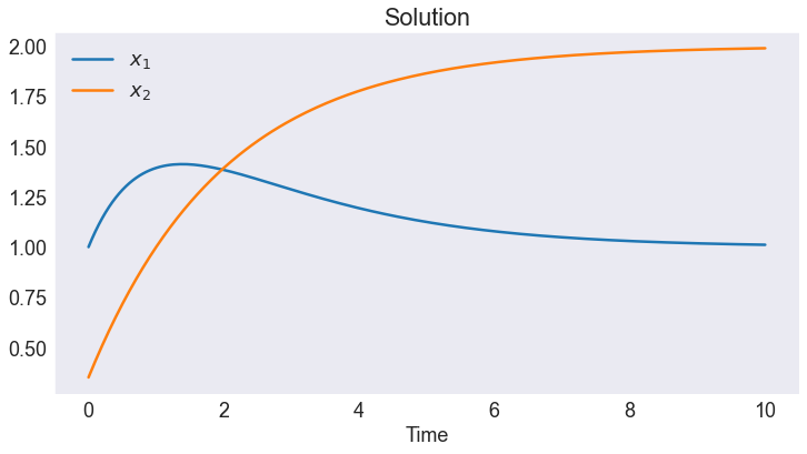
Closed-Form Solution
def X(t):
    values = np.array([1 - np.exp(1/2-t) + np.exp((1-t)/2), 2-np.exp((1-t)/2)])
    return pd.DataFrame(values.T, index=t, columns=xlabels)
SOLVE ODE ANALYTICALLY
# Time Discretization
N = 200                 # number of time nodes
t = np.linspace(0,T,N)  # time nodes

# Plot Closed-Form Solution in Time Domain
fig, ax = plt.subplots()
X(t).plot(ax=ax)
ax.set(title='Solution', xlabel='Time')
[Text(0.5, 1.0, 'Solution'), Text(0.5, 0, 'Time')]
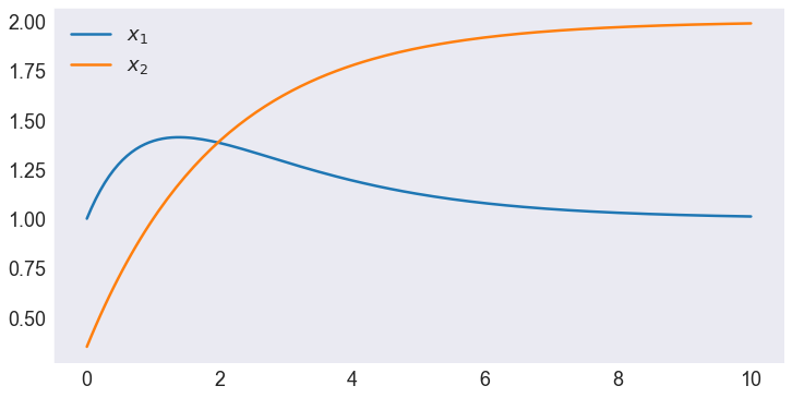
SOLVE ODE USING COLLOCATION METHOD
# Solve ODE
n = 15    # number of basis functions

problem = ODE(f, T, bv, A, b, labels=xlabels)
problem.solve_collocation(n=n, bt=bt, bx=bx, nf=10)

problem.x.plot()
<AxesSubplot:>
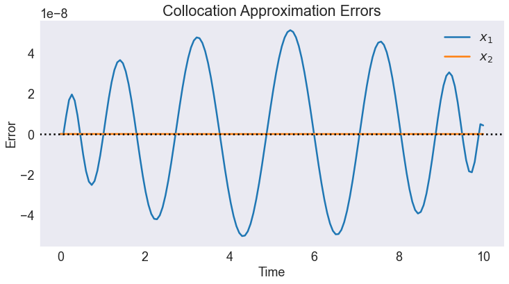
# Plot Collocation Approximation Errors
fig, ax = plt.subplots()

(problem.x - X(problem.x.index)).plot(ax=ax)
ax.axhline(0, color='black', ls=':')
ax.set(title='Collocation Approximation Errors',
       xlabel='Time',
       ylabel='Error');
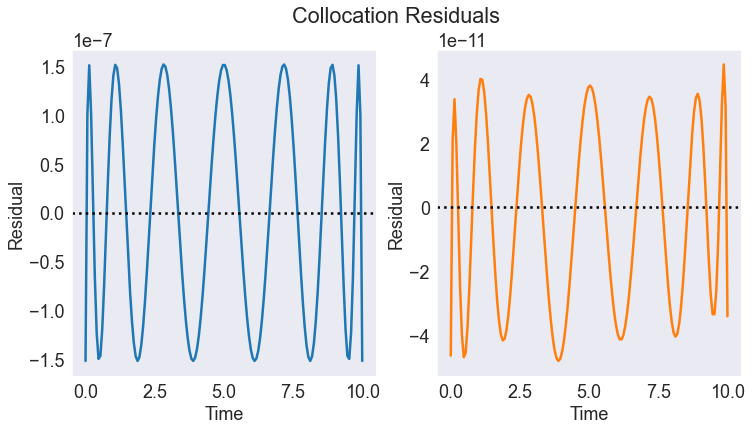
# Plot Residuals
fig, axs= plt.subplots(1,2)
problem.resid.plot(ax=axs, subplots=True, legend=False)

for ax in axs:
    ax.axhline(0, color='black', ls=':')
    ax.set(xlabel='Time', ylabel='Residual')


fig.suptitle('Collocation Residuals')
Text(0.5, 0.98, 'Collocation Residuals')
STEADY-STATE
# Compute Steady State
xstst = - np.linalg.solve(A,b)
print('Steady State')
print(xstst)
print('Eigenvalues')
print(np.linalg.eigvals(jacobian(f, np.atleast_2d(xstst).T, A, b)))
Steady State
[1. 2.]
Eigenvalues
[-1.  -0.5]
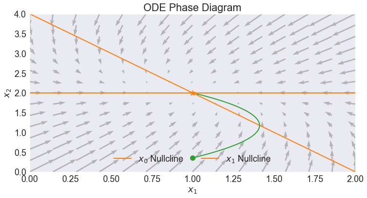
PHASE DIAGRAM
# Plotting Limits
x1lim = [0, 2]  # x1 plotting limits
x2lim = [0, 4]  # x2 plotting limits

# Compute Nullclines
x1 = np.linspace(*x1lim, 100)
xnulls = pd.DataFrame({'$x_0$ Nullcline': -(A[0,0]*x1 + b[0])/A[0,1],
                       '$x_1$ Nullcline': -(A[1,0]*x1 + b[1])/A[1,1]},
                     index = x1)

# Plot Phase Diagram
problem.phase(x1lim, x2lim,
         xnulls=xnulls,
         xstst=xstst,
         title='ODE Phase Diagram'
        )