Rational Expectations Agricultural Market Model
Contents
Rational Expectations Agricultural Market Model
Randall Romero Aguilar, PhD
This demo is based on the original Matlab demo accompanying the Computational Economics and Finance 2001 textbook by Mario Miranda and Paul Fackler.
Original (Matlab) CompEcon file: demintro02.m
Running this file requires the Python version of CompEcon. This can be installed with pip by running
!pip install compecon --upgrade
Last updated: 2022-Ago-19
import numpy as np
import pandas as pd
import matplotlib.pyplot as plt
from compecon import qnwlogn, discmoments
plt.style.use('seaborn-dark')
plt.style.use('seaborn-talk')
pd.set_option('display.precision', 4)
Generate yield distribution
sigma2 = 0.2 ** 2
y, w = qnwlogn(25, -0.5 * sigma2, sigma2)
Compute rational expectations equilibrium using function iteration, iterating on acreage planted
def A(aa, pp):
    """
    Parameters
        aa: acreage
        pp: target price
    """
    return 0.5 + 0.5 * np.dot(w, np.maximum(1.5 - 0.5 * aa * y, pp))

ptarg = 1.0 # target price
a = 1.0     # initial guess for acreage

print(f"{'it':^4s} {'a':^8s} {'|a-aold|':^8s}", '='*22, sep='\n')
for it in range(50):
    aold = a
    a = A(a, ptarg)
    print(f'{it:4d} {a:8.4f} {abs(a-aold):8.1e}')
    if abs(a - aold) < 1.e-8:
        break
 it     a     |a-aold|
======================
   0   1.0198  2.0e-02
   1   1.0171  2.7e-03
   2   1.0175  3.7e-04
   3   1.0174  5.0e-05
   4   1.0174  6.8e-06
   5   1.0174  9.3e-07
   6   1.0174  1.3e-07
   7   1.0174  1.7e-08
   8   1.0174  2.3e-09
Intermediate outputs
q = a * y                # quantity produced in each state
p = 1.5 - 0.5 * a * y    # market price in each state
f = np.maximum(p, ptarg) # farm price in each state
r = f * q                # farm revenue in each state
g = (f - p) * q          #government expenditures

varnames = ['Market Price', 'Farm Price', 'Farm Revenue', 'Government Expenditures']

data = pd.DataFrame(index=varnames, columns=['Expect', 'Std Dev'])
data['Expect'], data['Std Dev'] = discmoments(w, np.vstack((p, f, r, g)))
data
| Expect | Std Dev | |
|---|---|---|
| Market Price | 0.9913 | 0.1028 |
| Farm Price | 1.0348 | 0.0506 |
| Farm Revenue | 1.0447 | 0.1773 |
| Government Expenditures | 0.0573 | 0.1038 |
Generate fixed-point mapping
aeq = a
a = np.linspace(0, 2, 100)
g = np.array([A(k, ptarg) for k in a])
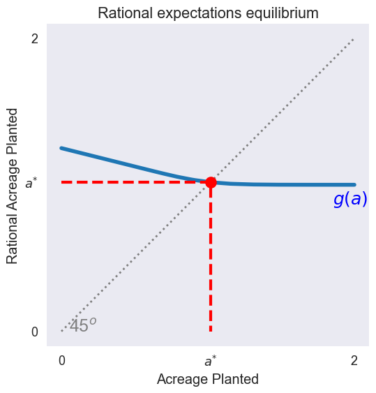
Graph rational expectations equilibrium
fig1, ax = plt.subplots(figsize=[6, 6])
ax.plot(a, g, linewidth=4)
ax.plot(a, a, ':', color='grey', linewidth=2)
ax.plot([0, aeq, aeq], [aeq, aeq, 0], 'r--', linewidth=3)
ax.plot([aeq], [aeq], 'ro', markersize=12)

ax.text(0.05, 0, '45${}^o$', color='grey')
ax.text(1.85, aeq - 0.15,'$g(a)$', color='blue')

ax.set(title='Rational expectations equilibrium',
       aspect=1,
       xlabel='Acreage Planted',
       xticks=[0, aeq, 2],
       xticklabels=['0', '$a^{*}$', '2'],
       ylabel='Rational Acreage Planted',
       yticks=[0, aeq, 2],
       yticklabels=['0', '$a^{*}$', '2']);
Compute rational expectations equilibrium as a function of the target price
def solve_farm_problem(ptarg):
    a=1.0 # initial guess

    for it in range(50):
        aold = a
        a = A(a, ptarg)
        if abs(a - aold) < 1.e-10:
            break

    q = a * y                       # quantity produced
    p = 1.5 - 0.5 * a * y           # market price
    f = np.maximum(p, ptarg)    # farm price
    r = f * q                       # farm revenue
    g = (f - p) * q                 # government expenditures

    return discmoments(w, np.vstack((p, f, r, g)))


nplot = 50
ptargets = np.linspace(0, 2, nplot)

E = pd.DataFrame(index=ptargets, columns=varnames)
S = pd.DataFrame(index=ptargets, columns=varnames)
E.index.name = 'Target price'
S.index.name = 'Target price'


for ptarg in ptargets:
    E.loc[ptarg], S.loc[ptarg] = solve_farm_problem(ptarg)
Graph expected prices vs target price
zeroline = lambda y, ax: ax.axhline(y.iloc[0], linestyle=':', color='gray')

fig2, (ax1,ax2) = plt.subplots(1, 2, figsize=[8, 6])

zeroline(E['Market Price'], ax1)
E[['Market Price','Farm Price']].plot(ax=ax1, linewidth=4)
ax1.set(title='Expected price',
        xticks=[0, 1, 2],
        ylabel='Expectation',
        yticks=[0.5, 1, 1.5, 2],
        ylim=[0.5, 2.0])

ax1.legend(loc='upper left')

# Graph expected prices vs target price
zeroline(S['Farm Price'], ax2)
S[['Market Price','Farm Price']].plot(ax=ax2, linewidth=4)
ax2.set(title='Price variabilities',
        xticks=[0, 1, 2],
        ylabel='Standard deviation',
        yticks=[0, 0.1, 0.2])

ax2.legend(loc='upper left');
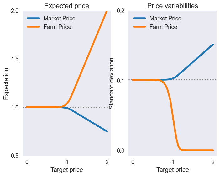
fig3, (ax1, ax2, ax3) = plt.subplots(1, 3, figsize=[12, 6])

# Graph expected farm revenue vs target price
zeroline(E['Farm Revenue'], ax1)
E['Farm Revenue'].plot(ax=ax1, linewidth=4)
ax1.set(title='Farm revenue',
        xticks=[0, 1, 2],
        ylabel='Expectation',
        yticks=[1, 2, 3],
        ylim=[0.8, 3.0])

# Graph standard deviation of farm revenue vs target price
zeroline(S['Farm Revenue'], ax2)
S['Farm Revenue'].plot(ax=ax2, linewidth=4)
ax2.set(title='Farm Revenue Variability',
        xticks=[0, 1, 2],
        ylabel='Standard deviation',
        yticks=[0, 0.2, 0.4])

# Graph expected government expenditures vs target price
zeroline(E['Government Expenditures'], ax3)
E['Government Expenditures'].plot(ax=ax3, linewidth=4)
ax3.set(title='Expected Government Expenditures',
        xticks=[0, 1, 2],
        ylabel='Expectation',
        yticks=[0, 1, 2],
        ylim=[-0.05, 2.0]);
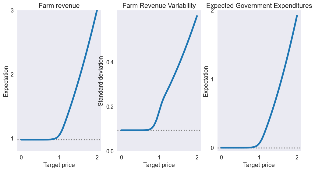
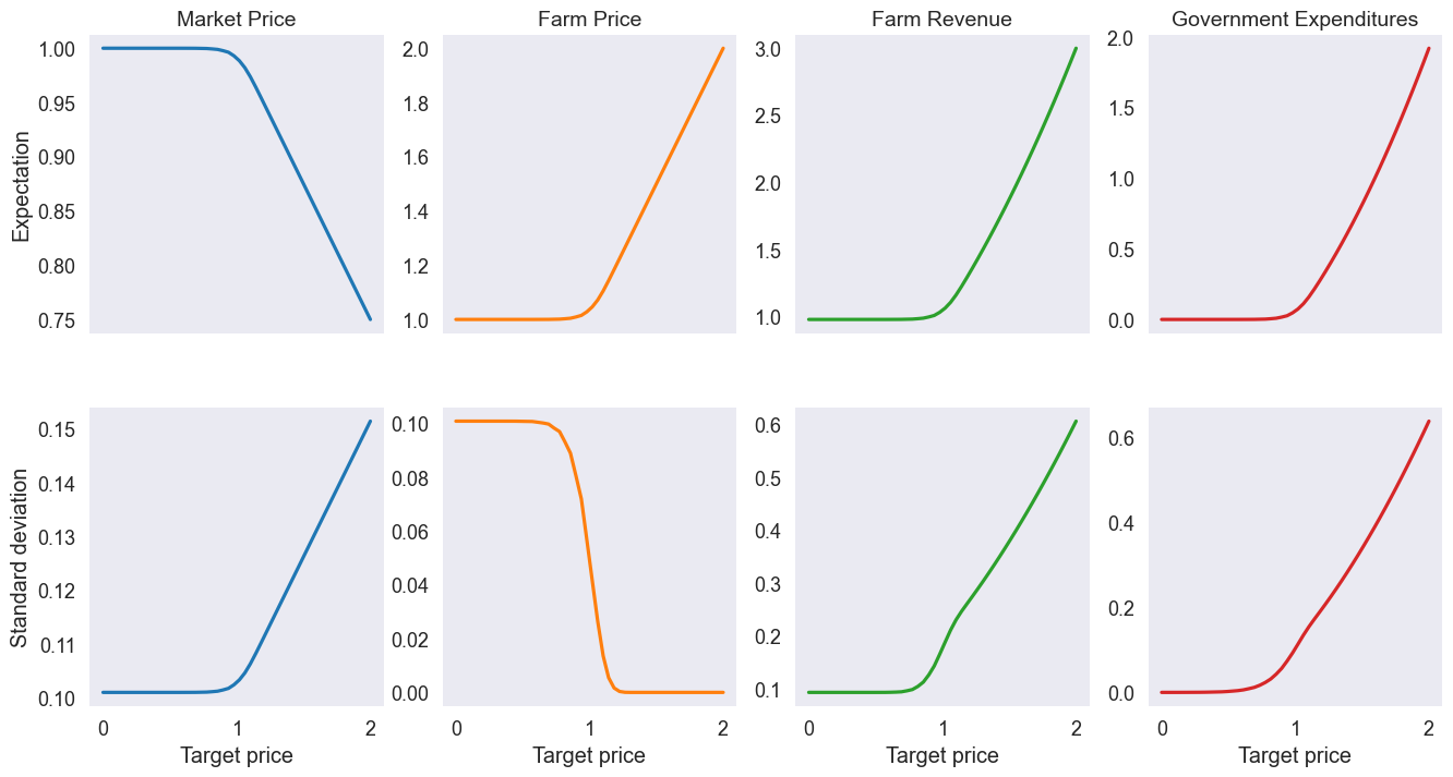
fig4, axs = plt.subplots(2, 4, figsize=[16,8], sharex=True)
E.plot(subplots=True, ax=axs[0], legend=None);
S.plot(subplots=True, ax=axs[1], legend=None);

for ax, tlt in zip(axs[0], E):
    ax.set_title(tlt, size=14)

axs[0,0].set_ylabel('Expectation')
axs[1,0].set_ylabel('Standard deviation')
Text(0, 0.5, 'Standard deviation')