Approximating Runge’s function
Contents
Approximating Runge’s function
Randall Romero Aguilar, PhD
This demo is based on the original Matlab demo accompanying the Computational Economics and Finance 2001 textbook by Mario Miranda and Paul Fackler.
Original (Matlab) CompEcon file: demapp04.m
Running this file requires the Python version of CompEcon. This can be installed with pip by running
!pip install compecon --upgrade
Last updated: 2022-Oct-22
About
Uniform-node and Chebyshev-node polynomial approximation of Runge’s function and compute condition numbers of associated interpolation matrices
Initial tasks
import numpy as np
import matplotlib.pyplot as plt
from numpy.linalg import norm, cond
from compecon import BasisChebyshev
import warnings

warnings.simplefilter('ignore')
Runge function
runge = lambda x: 1 / (1 + 25 * x ** 2)
Set points of approximation interval
a, b = -1, 1
Construct plotting grid
nplot = 1001
x = np.linspace(a, b, nplot)
y = runge(x)
Plot Runge’s Function
Initialize data matrices
n = np.arange(3, 33, 2)
nn = n.size
errunif, errcheb = (np.zeros([nn, nplot]) for k in range(2))
nrmunif, nrmcheb, conunif, concheb = (np.zeros(nn) for k in range(4))
Compute approximation errors on refined grid and interpolation matrix condition numbers
for i in range(nn):
    # Uniform-node monomial-basis approximant
    xnodes = np.linspace(a, b, n[i])
    c = np.polyfit(xnodes, runge(xnodes), n[i])
    yfit = np.polyval(c, x)
    phi = xnodes.reshape(-1, 1) ** np.arange(n[i])

    errunif[i] = yfit - y
    nrmunif[i] = np.log10(norm(yfit - y, np.inf))
    conunif[i] = np.log10(cond(phi, 2))

    # Chebychev-node Chebychev-basis approximant
    yapprox = BasisChebyshev(n[i], a, b, f=runge)
    yfit = yapprox(x)  # [0] no longer needed?  # index zero is to eliminate one dimension
    phi = yapprox.Phi()
    errcheb[i] = yfit - y
    nrmcheb[i] = np.log10(norm(yfit - y, np.inf))
    concheb[i] = np.log10(cond(phi, 2))
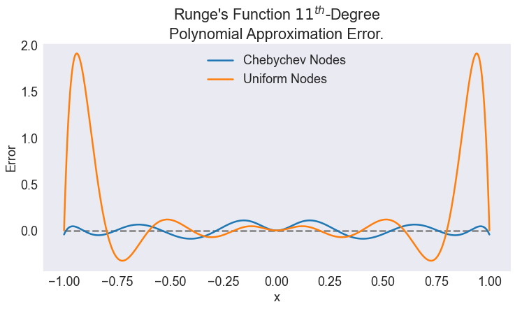
Plot Chebychev- and uniform node polynomial approximation errors
fig1, ax = plt.subplots()
ax.plot(x, y)
ax.text(-0.8, 0.8, r'$y = \frac{1}{1+25x^2}$', fontsize=18)
ax.set(xticks=[], title="Runge's Function", xlabel='', ylabel='y');
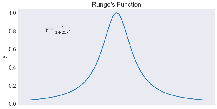
fig2, ax = plt.subplots()
ax.hlines(0, a, b, 'gray', '--')
ax.plot(x, errcheb[4], label='Chebychev Nodes')
ax.plot(x, errunif[4], label='Uniform Nodes')
ax.legend(loc='upper center')
ax.set(title="Runge's Function $11^{th}$-Degree\nPolynomial Approximation Error.", xlabel='x', ylabel='Error')
[Text(0.5, 1.0, "Runge's Function $11^{th}$-Degree\nPolynomial Approximation Error."),
 Text(0.5, 0, 'x'),
 Text(0, 0.5, 'Error')]
Plot approximation error per degree of approximation
fig3, ax = plt.subplots()
ax.plot(n, nrmcheb, label='Chebychev Nodes')
ax.plot(n, nrmunif, label='Uniform Nodes')
ax.legend(loc='upper left')
ax.set(title="Log10 Polynomial Approximation Error for Runge's Function",xlabel='', ylabel='Log10 Error', xticks=[])
[Text(0.5, 1.0, "Log10 Polynomial Approximation Error for Runge's Function"),
 Text(0.5, 0, ''),
 Text(0, 0.5, 'Log10 Error'),
 []]
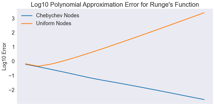
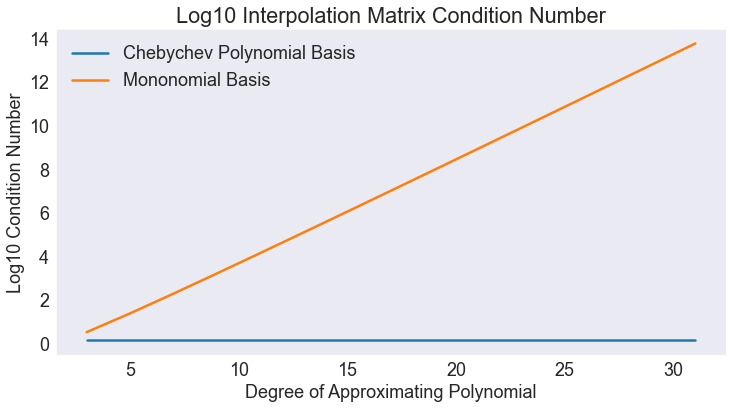
fig4, ax = plt.subplots()
ax.plot(n, concheb, label='Chebychev Polynomial Basis')
ax.plot(n, conunif, label='Mononomial Basis')
ax.legend(loc='upper left')
ax.set(title="Log10 Interpolation Matrix Condition Number",
       xlabel='Degree of Approximating Polynomial',
       ylabel='Log10 Condition Number')
[Text(0.5, 1.0, 'Log10 Interpolation Matrix Condition Number'),
 Text(0.5, 0, 'Degree of Approximating Polynomial'),
 Text(0, 0.5, 'Log10 Condition Number')]